
Posted by Christine Obbink-Huizer
Categories
solving non convergence with Abaqus FEATable of contents
Every engineer trying to solve non-linear finite element analyses has experienced it: convergence difficulties. In this blog I will give ideas for finding the cause of the convergence issues, as well as some common solutions in Abaqus FEA.
1) Check the Job Diagnostics
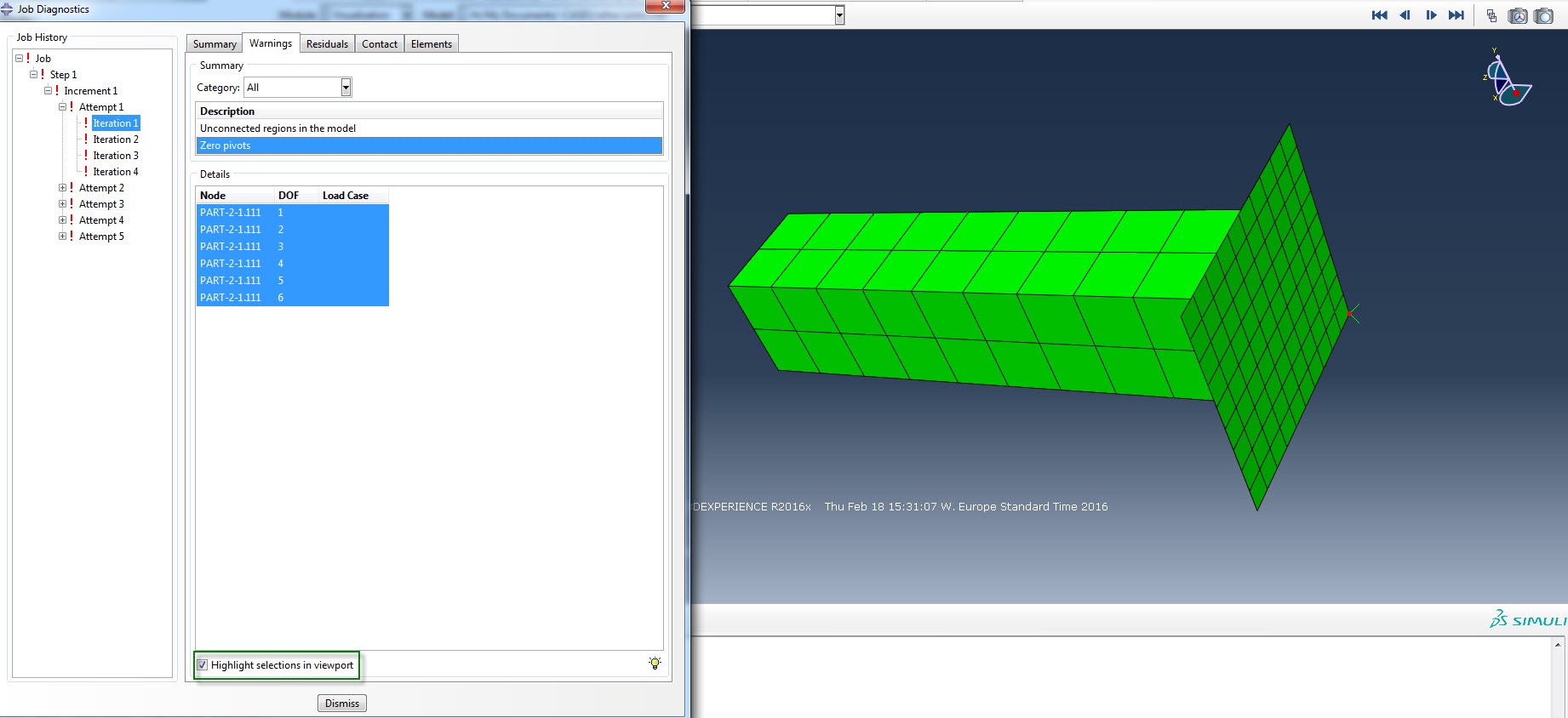
Open the odb and select tools>job diagnostics. Job diagnostics gives all warnings and errors, as well as residual and contact information. One of the most useful features is the highlight selection in viewport check box.
In the warnings tab, the user can see the location of numerical singularities and zero pivots (if applicable), which may give an idea of what causes these warnings.
In the residuals tab, the node with the largest residual can be visualised. Looking at this node for the iteration that convergence difficulties arise, often shows the region of the model that is causing problems. Is anything unexpected happening in this region?
In the contact tab the location of the maximum contact force error and the maximum penetration error can be viewed. If contact is causing the problems, this will likely show where.
2) Pay Attention to Warning Messages
Look at when the warning is issued and whether it is likely to point towards the problem. For example, if the solver tries a first attempt with a big increment and gives a warning related to a negative eigenvalue and then cuts back the time increment and obtains convergence in the next increments without any difficulties or warnings, it is likely that the warning was simply a consequence of trying a too big time step. If the warning message repeats itself and repeated cut-backs occur, it may indicate a stability issue (see point 6).
Some warnings are very specific, others can occur with different underlying causes and require more experience to work out the problem.
3) Check Boundary Conditions
One cause of non-convergence is inadequate boundary conditions. Unreasonable boundary conditions can lead to local extreme deformations. A model can also be over or under constrained. With an under constraint, not all rigid body motion is suppressed, leading to one or more degrees of freedom with zero stiffness and usually zero-pivot warnings. Over constraints also tend to cause zero-pivot warnings. Though Abaqus checks for over constraints and tries to solve them, this is not always possible, for example if the over constraint starts occurring after some time due to contact. It is recommended to check all warning messages related to over constraints. Do not assume Abaqus will correctly resolve the over constraint, but correctly define the constraint yourself. Also, look at the location of zero-pivot warnings (are there over or under constraints there?).
4) Check Contact
Contact is also a major contributor to convergence difficulties. Come to think of it, this is not so strange, as the onset of contact gives a discontinuity in the force-displacement relationship, which increases the difficulty of finding a solution with Newton’s method. That’s why Abaqus uses separate severe discontinuity iterations when contact is changing.
One possible source of contact non-convergence is the initial state of the contact. If a problem relies on the contact for stability and initially no contact is present, the simulation may have trouble starting. This is especially the case load control is used: basically a load is applied to something without a stiffness and rigid body motion can occur. (Initially) using displacement control to ensure contact occurs usually resolves the convergence issues. Abaqus also offers contact stabilization to help automatically control rigid body motion in static problems before contact.
This can be defined within contact controls, by using automatic stabilization. It is necessary to specify that the contact controls are to be used in the interaction definition. With automatic stabilization, damping is applied when the surfaces are close to each other but not in contact, so there is a resistance to displacement of the loaded part and rigid body motion is no longer possible. Because this is meant to allow surfaces to get into contact, the damping is ramped down, by default to 0, during the step in which it is applied. It is recommended to check if viscous dissipation is not too large, e.g. compare ALLSD to ALLIE. The techniques to resolve instabilities mentioned in point 6 can also be applied.
Another potential source of contact non-convergence is that no contact is defined for surfaces which are actually in contact, which can lead to unrealistic results, very large deformations and non-convergence. A self-contact can for example easily be overlooked. This normally does not happen when Abaqus’ powerful general contact is applied.
5) Check Material Definition
Convergence issues can occur when the stress in the material does not increase when the strain increases (the stiffness is not positive). This could happen when experimental data including damage are used to define the model, without including a damage model. Check the (maximal) stresses and strains in the model to see whether damage is expected to occur.
If Abaqus’ material fitting options for hyperelastic models are used, there may be limits to the stability of the material. By right-clicking on the material and selecting ‘evaluate’ it is possible to view the stability limits calculated by Abaqus.
When a plastic material model is used and the loading reaches the end of the defined curve, Abaqus extrapolates the curve with a horizontal line: the (plastic) strain can increase, but the stress does not (perfect plasticity). The stiffness is zero in this case. If this happens in a single element, often the simulation will run without problems. When large parts of the model undergo perfect plasticity it can become a problem. This often indicates the load is too much for the material.
6) include Damping to Resolve Instabilities
Possibly the most common cause of non-convergence is the presence of an instability. One of the principles of model development, is that a model should not be more complex than necessary to describe the behaviour of interest. With this in mind, it seems reasonable to decrease the complexity of a model by assuming it behaves statically, when the process is slow. Interestingly, however, this simplification can make the model more difficult to solve. In general, the behaviour of material under load is described by Newton’s second law:
F= m x a (force equals mass times acceleration)
When static behaviour is assumed, the acceleration equals zero, so the sum of all forces must equal zero: there is force equilibrium. The static assumption is valid when the system moves from one equilibrium state to the next and all in between states are also in equilibrium. But is this always the case?
Take the example of two parts not initially in contact with load control. Why is this situation possible in reality? Because the initial displacement of the loaded part will be determined by its inertia. The inertia, the effect we had simplified out, actually stabilizes the problem. Including some kind of inertia or damping effect can often help to obtain a converged solution. There are several methods to do this.
Within the step definition, automatic stabilization can be chosen, e.g. with the default specify dissipated energy fraction.

This applies an extra viscous force, proportional to the nodal displacement divided by the time step to all nodes in the model, which has a stabilizing effect. Check if viscous dissipation is not too large, e.g. compare ALLSD to ALLIE.
An alternative is to use a dynamic, implicit step. As application quasi-static can be chosen.

This uses an Euler Backward scheme, which has a viscous effect that is based on the real mass. In this case a time-dependent problem is solved, so the time scale should be reasonable. Check whether the kinetic energy is small with respect to the internal energy.
And If Nothing Works?
Try Explicit. Though the simulation may take long, in some extremely non-linear cases it is just not realistic to obtain a converged solution with Abaqus/Standard. With Abaqus/Explicit, at least you can be certain you won’t have any convergence issues.
And who knows? It may be more efficient to let your computer spend more time solving your actual problem, than to keep modifying the model hoping that this last change will be the trick that gets you to the end of the step.
Are you ready to throw the towel in the ring and need help with your convergence challenge?


TECHNIA Simulation provides top tier FEA, Non-linear, and Advanced Simulation Software, Training, and Consultancy. Our dedicated team of more than 65 Simulation experts across 16 countries advise and support your innovation with a wealth of specialist knowledge and experience.
About TECHNIA- Related news and articles straight to your inbox
- Hints, tips & how-tos
- Thought leadership articles

Helping you find the information you’re looking for. Discover webinars, events, FAQ's, case studies and tutorials.
VIEW HUB