
Posted by Nikolaos Mavrodontis
Table of contents
In this blog, we will describe the possibilities for Buckling and the methodology to take into account imperfections.
Buckling refers to the sudden collapse of a structural member , subjected to high axial compressive loading. This collapse takes the form of a sudden lateral deflection of the structural member. Therefore the structure’s load bearing ability is compromised under buckling. Based on the structure’s characteristics, either a consequent full collapse can occur or the structure’s load bearing capacity is restored in the post-buckled region. When the structure exhibits this sudden lateral deflection under axial compression, it is said that the buckling load has been reached. The importance of considering buckling during structural design is outlined by the fact that the buckling load is lower than the maximum load the structure can withstand under axial compression.
Typically slender structures such as columns, trusses, shells and plates are buckling-prone structures. The buckling instability is the result of purely geometrical effects and it does not relate to other forms of non-linearity (e.g. material non-linearity).
When an axisymmetric structure (e.g. a cylinder) is subjected to axial compression, under increasing load there comes a critical load value (Pcritical) after which the structure’s response can only take the form of two states in equilibrium. Either a purely compressed state –therefore not exhibiting any lateral deflection- or a laterally deformed state. This point is called a bifurcation point. This form of discontinuity prevents in many occasions achieving of convergence for solvers in finite element analyses.
A structure's behavior under loading is usually studied with the use of load-displacement plots. This applies also to studying the structural behavior in the post-buckling region (past the bifurcation point). Two relevant plots (one for in plane and one for out of plane displacement) for a shell structure (e.g. a chimney with a circular cross section, a monopile structure etc.) are given below.
Load vs in plane displacement q
Shell structures (structures the thickness of which is relatively small compared to its other dimensions), exhibit a post buckling behavior where negative stiffness occurs accompanied by a sudden load-bearing reduction. See picture below.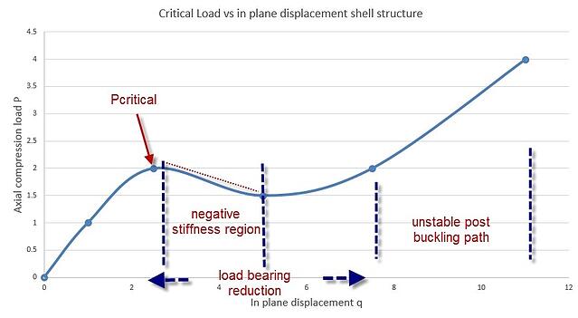
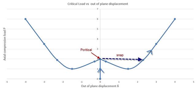
Load vs out of plane displacement δ
For a shell structure under axial compression when the critical load is reached , the structure instantly loses its load bearing capacity and exhibits a significant lateral displacement δ (snap). This lateral motion can be quite localized. On each of the secondary paths, the structure exhibits sudden high lateral displacements, jeopardizing its stability as well as its load bearing ability.
At this point the structure releases membrane strain energy (accumulated by the axial load) in the form of kinetic energy. In the post buckling region after a certain value of lateral displacement has been reached, the structure regains its load-bearing capacity and can be loaded further over its critical load value. See picture below.
From the example above, it can be concluded that a structure’s behavior in the post-buckling region is of crucial importance for designers and engineers. Different types of buckling-prone structures, exhibit different behaviors in the post-buckling regions.
Abaqus offers various types of analyses, focusing on capturing the post buckling behavior, such as the Riks analysis. This type of analysis usually succeeds a linear buckle load analysis and is based on introducing an imperfection to the structure. An example is given:
Linear Buckle Analysis
Geometry
The geometry consists of a thin walled (shell) cylinder under a compressive unit load in order to find the buckling load corresponding to the 1st mode
Imperfections request
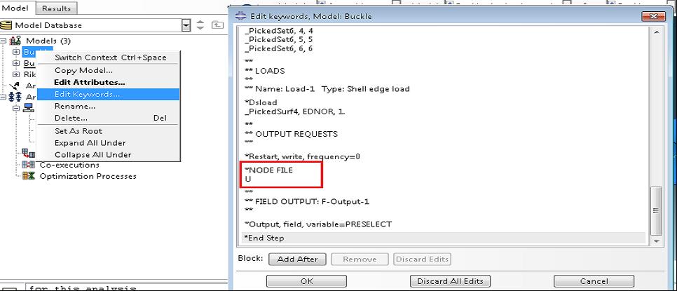
Prior to submitting the buckling analysis job (Subspace solver was used-smaller run times when only a few modes are requested), the node coordinates for the different mode shapes must be written as output. This procedure is shown below. This output will be consequently introduced as imperfections for the Riks analysis so as to achieve a smoother transition to the post buckling region and surpass the bifurcation problem.
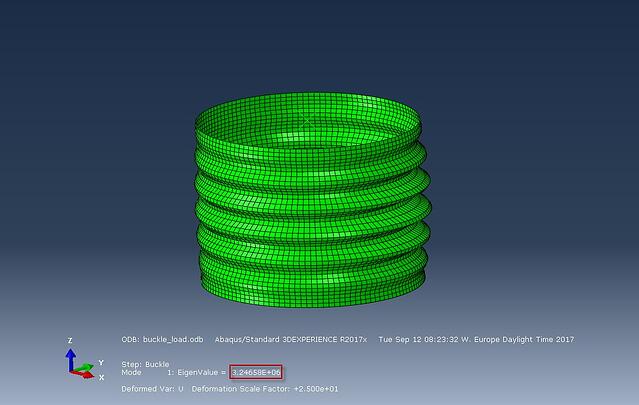
Results linear buckle analysis
The predicted linear buckle load for the 1st mode is given below:
Riks Analysis
For the Riks analysis, minor modifications must be performed to the model. The NLGEOM flag must be turned on to account for non-linearities. Additionally the unit compressive load must be replaced by the buckling load value predicted by the linear buckle analysis.
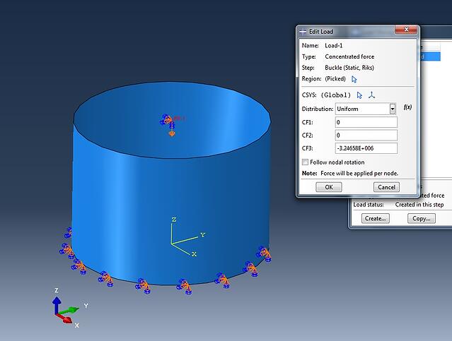
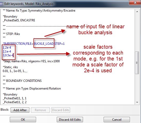
Last but not least the imperfections must be introduced for the Riks analysis. This is done again by editing the model΄s keywords.

Each scale factor corresponds to a scaled shape of each mode (nodal displacements are scaled down). For choosing an appropriate scale factor, a good rule of thumb, is to choose an order of magnitude lower than the shell thickness for the 1st mode (most important of modes) and decrease the subsequent scale factor by half of the first scale factor.
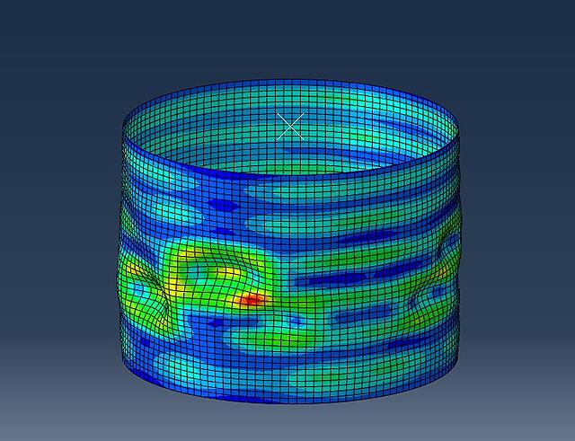
Results Riks Analysis
Below the stress contours are shown. It can be seen that the structure is at the post buckled region.
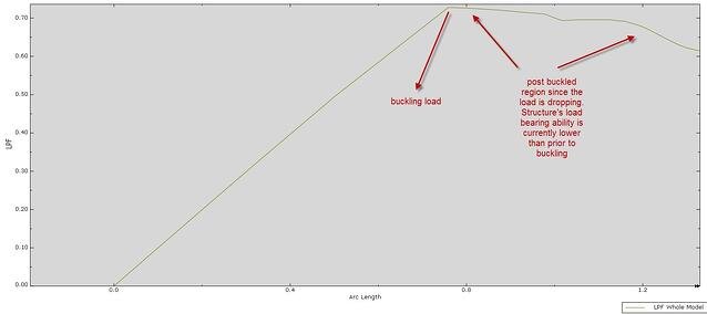
By plotting the Load proportionality factor (LPF) we can trace the prebuckling and post buckling regions based on the load applied be the Riks algorithm.
Conclusions and Remarks
As demonstrated, the Riks algorithm is a powerful tool for assessing a structure’s behavior in the post-buckling region. By introducing imperfections (either by mesh perturbation or by scaled mode shapes-as performed here-) we achieve a smoother transition to the post-buckling region. The example shown above can be applied when investigating the behavior of imperfection-sensitive structures.
Are you not experienced enough yet, to perform these analyses yourself?


TECHNIA Simulation provides top tier FEA, Non-linear, and Advanced Simulation Software, Training, and Consultancy. Our dedicated team of more than 65 Simulation experts across 16 countries advise and support your innovation with a wealth of specialist knowledge and experience.
About TECHNIA- Related news and articles straight to your inbox
- Hints, tips & how-tos
- Thought leadership articles

Helping you find the information you’re looking for. Discover webinars, events, FAQ's, case studies and tutorials.
VIEW HUB