

Posted by Christine Obbink-Huizer
Table of contents
When performing a finite element analysis many modelling choices must be made. One of them is the choice of material properties. This can have a big influence on the outcome of the simulation. In many cases some material properties are known, for example in a data sheet. These normally do not directly correlate to the parameters required by Abaqus. When not all the required material properties are known, experimental data must be obtained. Based on this data, a material model and material parameters must be defined.
Material Calibration in Abaqus
Within Abaqus, there are some possibilities to do this. For elastic-plastic materials a calibration can be performed based on stress-strain data from uniaxial elongation. For hyperelastic materials, an evaluation can be performed. In this case, material parameters are estimated for different material models, based on uniaxial, biaxial, planar and/or volumetric test data using a one element model. The estimated stress-strain graph(s) can be compared to the experimental one(s) and based on this, the material model with the best fit can be chosen.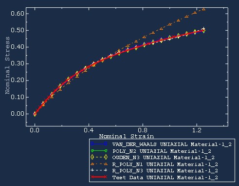
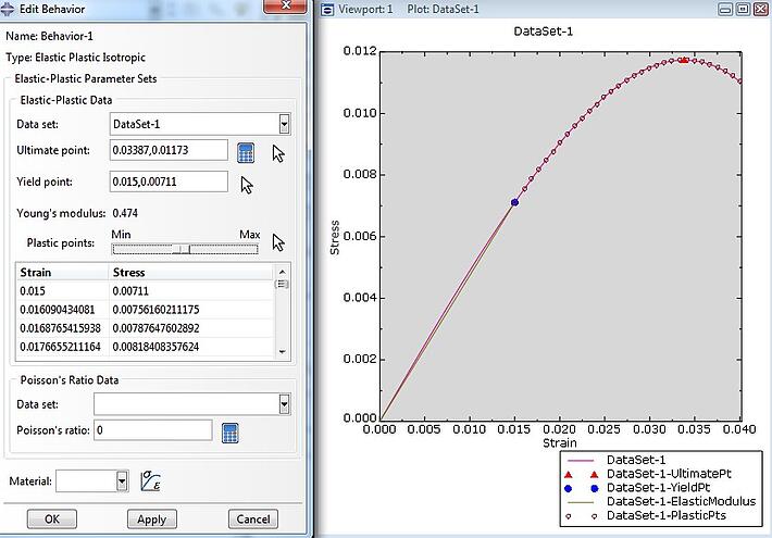
Figure 2: Material calibration.
Manual Calibration Using Abaqus
These options require standard tests to be performed. This is not always practical or representative of the loading applied in practice. In these cases, Abaqus can be used to calibrate material data. To do this, you need experimental data and a simulation of the experimental set-up. Experimental and simulated results are then compared to determine how good the fit is. If the fit is not satisfying, the material properties are modified and the simulation is rerun, trying to obtain a better fit. This can be done manually, but it is labour intensive. Also, it can be difficult to determine how the material properties should be modified to try to obtain a better fit. Isight can automate this process while allowing use of a predefined optimization algorithm.
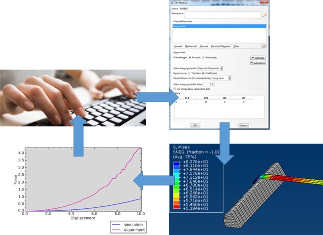
Figure 3: Manual calibration loop.
Using Isight and Abaqus for Material Calibration
Setting up Abaqus
When using Isight to calibrate the material properties, the main approach is similar to the manual approach: you still need experimental data and a model of the experiment in Abaqus. Because this model will be run several times, it makes sense to pay attention to things that might speed up the simulation, such as using symmetry conditions or assuming parts are rigid.
When using Abaqus with Isight, they must communicate with each other: Abaqus must receive material parameters from Isight (input) and send results to be compared to experimental results back (output). By default, material parameters are available as input, so no modifications are required for this. It is necessary to define output in the simulation in such a way so that it can be compared to the available experimental data, possibly after post processing with a python script.
After setting up the model in Abaqus, it must be run once to obtain an .odb, from which the output can be extracted. Abaqus can then be closed.
Setting up Isight
The next step is to set up Isight. The Isight model of course contains an Abaqus component. It refers to the Abaqus model (.cae or .inp) and results (.odb) files. The input parameters (in this case the material properties) and output parameters (in this case e.g. force and displacement for comparison to experimental data) can be specified by checking them in a list of available parameters.
Besides the Abaqus component, a Data Matching component is used. In this component, the experimental data is specified, as well as the outputs that are to be compared to it and the measure that will be used to describe how good the fit is (such as the sum of the squared differences between simulation and experiment). With these two components, we can perform a simulation for specific material properties and determine how well the results match experimental results, but we do not change material properties to obtain a better match yet.
This is done with an Optimization component. Different algorithms for optimization are available, in three categories: direct, gradient based and exploratory algorithms. Exploratory algorithms look for a global optimum. This is more computationally expensive than looking for a local optimum. Direct and gradient based techniques search for a local optimum. This is generally much faster, but the result depends on the starting point. As the name suggests, gradient based techniques use a derivative to determine the searching location. Because of this, they do not work well with discontinuous functions. Direct techniques do not have this limitation.
It can be valuable to run the Isight model using different optimization techniques and/or starting points to find a good solution within a reasonable amount of time. When selecting an optimization technique, Isight provides information on the technique, including the type of problems it is or is not suitable for. This can help choosing from one of the many possibilities. Not only an algorithm, but also an optimization criterion (e.g. minimize the summed squared difference) and a termination criterion (such as the difference being less than a certain value) are specified.
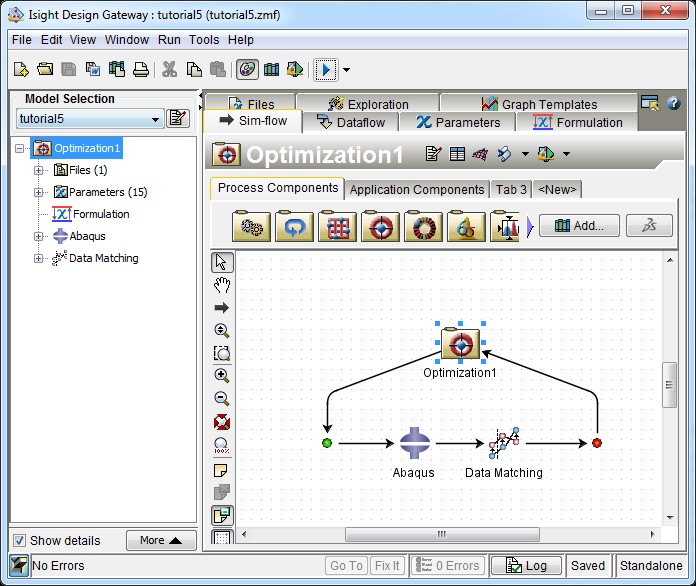
Figure 4: Running the analysis from within an integrated Isight loop.
After the Isight model is set up, it can be run. This will take some time, as the Abaqus simulation must be run several times. While Isight is running, information on the current parameter values is shown, highlighting the currently found best solution. This allows monitoring of the process.
Isight has many different options to visualise results, including histograms, history graphs, scatter plots and surface plots allowing visualisation of the relationship between different input and output parameters. These can be defined beforehand, so they are created as the analysis is run. In this example of material calibration, we are probably interested in relatively simple outcomes such as the final values of the material parameters and a visual comparison of experimental and simulated data.
Try It Yourself?
Want to try material calibration with Abaqus and Isight? Get started by looking at our Isight Tutorials.


TECHNIA Simulation provides top tier FEA, Non-linear, and Advanced Simulation Software, Training, and Consultancy. Our dedicated team of more than 65 Simulation experts across 16 countries advise and support your innovation with a wealth of specialist knowledge and experience.
About TECHNIA- Related news and articles straight to your inbox
- Hints, tips & how-tos
- Thought leadership articles

Helping you find the information you’re looking for. Discover webinars, events, FAQ's, case studies and tutorials.
VIEW HUB