Use Submodeling in Abaqus to Focus on Region of Larger Model

In some cases results of interest are on different length scales. The overall behaviour of a product is of interest, but also the detailed behaviour of a specific part. It is possible to create a locally refined mesh, but this is often time consuming. Meshing will be more troublesome and the computational cost can significantly increase with a more refined mesh. Also, it is not always known in advance exactly which region should be refined.

An alternative is to use submodeling. First the complete model is analysed, usually with a relatively coarse mesh. To get more detailed information on the specific part, results from the complete model can be used to define boundary conditions for the part. This is also a suitable approach when it is not possible to determine the boundary conditions on the part, without taking into account the rest of the product. In this blog I will explain what Abaqus does when the submodeling capabilities are invoked, show how easy it is to set up an analysis using submodeling and discuss the things you need to pay attention to yourself.

Concept

The idea behind submodeling is actually quite simple: a ‘big’ (global) model is used to generate boundary conditions in a ‘smaller’ (sub-) model. With ‘boundary conditions’ I literally mean conditions at the boundary in this case. These can either be node-based or surface-based. For the node-based option, global nodal results are interpolated onto submodel nodes, so boundary conditions in the traditional sense are defined. For the surface-based option, the global stress field is interpolated to obtain a surface traction that is applied to the submodel surface at the boundary. This is literally a condition at the boundary; in the terms used by Abaqus this is a load and not a boundary condition. We will see later on that indeed node-based submodeling is defined as boundary condition, and surface-based submodeling is defined as load.

Node-base Versus Surface-based Submodeling

Node-based submodeling is the more general and common option. It is available for different step types and not only for solid-to-solid coupling, but also for shell-to-shell and even shell-to-solid coupling amongst other options. Surface-based submodeling is only available for solid-to-solid submodeling in static, general analysis steps. If surface-based submodeling is used to define loads and boundary conditions in the model and no other boundary conditions are applied, then rigid body modes leading to convergence difficulties may occur. In this case using inertia relief may be a solution.

Choosing a Submodeling Technique

When wanting to use submodeling for anything but solid-to-solid coupling using a static general step, the choice of technique is easily made, as only node-based submodeling is available. Surface-based submodeling is most useful when the simulation is load-controlled (so the primary loading is through forces and/or pressures and not via displacements) and there are stiffness changes between the global model and the submodel. Such stiffness changes can occur due to changes in material properties or geometry, e.g. additional holes. In other cases the node-based technique tends to give similar results, without the chance of having numerical issues due to rigid body modes. Large displacements and rotations are more accurately transmitted using node-based submodeling. Both techniques can be combined in a single model.

Example: Roof Construction

I will now show how to set up an analysis using submodeling. The analysis of a roof construction is used as example. One of the joints will be analysed in more detail using a submodel (Figure 1). Separate models need to be defined for the global and submodel analysis. The results from the global model will be used to apply end conditions to the submodel.

Figure 1: Roof construction. Only a quarter (non-transparent) is modelled for reasons of symmetry. The joint indicated with a red oval will be analysed in more detail using a submodel.

Global Model

The first step is to set up the global model. This is done the same way a model is normally set up. The only thing to pay attention to so you will be able to use the results to drive the submodel later on, is to request the relevant results in the region of interest. For node-based submodeling this will usually be displacements and for surface-based submodeling this is stress. In this example, the default output requests for the whole model are unchanged, providing both displacement and stress. Output is requested at fixed time points with increments of 0.05 s (step time is 1 s) so the boundary conditions for the submodel will be known at these points and the resolution in time is sufficient.
The different parts used in the analysis are indicated in Figure 2.

Figure 2: Parts used. Some separation is applied, to make the different parts more clearly visible. Each part is indicated with a different colour. The mesh is also shown.

Material properties are based on wood. The actual complexity, such as anisotropy, is not taken into account for this simple example. Instead, isotropic linear elasticity is assumed. The stiffness of the roof (red part in Figure 2) is increased, to simulate stiffening constructions that would be there in practice.

A not-too-fine mesh (visible in Figure 2) is used for this global model. It has at least four elements through the thickness. Linear reduced integration elements are used, solids for everything but the roof and shells for the roof. The different parts are connected to each other via ties. For the submodel, this will be changed to a bolt-like construction.

A gravity loading is applied to the whole model. Symmetry conditions are applied as appropriate. The top and bottom of the roof cannot move downward, to simulate them resting on beams. Two beam ends are complete constrained, to model where the roof is fixed to the rest of the house (Figure 3).

Figure 3: Boundary conditions

This simulation is run, and results are obtained (Figure 4). Deformations are larger than would be expected in reality, this is to obtain more clearly visible results.

Figure 4: Deformed shape and Mises stress in global model

Submodel

Remove Unnecessary Geometry

 
Figure 5: Submodel after cutting and removal of unnecessary parts.

Add Additional Detail if Required

It is possible to add additional detail on the submodel compared to the global model. In fact, because the only thing Abaqus does with the submodeling technique is apply boundary conditions, we can make almost any modification we want. Abaqus will still apply the displacement or stress at the specified position in the global model to the same position in the submodel, even if there is no connection between the models whatsoever and using the submodeling technique does not make sense. Because Abaqus does not check whether the applied conditions are reasonable, the analyst needs to ensure this.

In this example, I’ve added additional holes and bolt-like structures to simulate the connection between the beams (Figure 6). The previously used ties are suppressed, and general contact is included.

Figure 6: Submodel geometry.

Remesh

The submodel needs to be meshed. Because the geometry is changed (regions are cut off, possibly detail included) in most cases the previously used mesh will not be usable any more. Even if the geometry would not require a remesh, usually submodelling is used to obtain more detailed results and a finer mesh is required.

In this case, a more refined mesh is used (Figure 7).

Figure 7: Global and submodel mesh.

Apply Loads and Boundary Conditions

With the geometry in place, the loads and boundary conditions that cause the submodel to be driven by the global model can be defined. These are defined similar to the way other loads or boundary conditions would.

Node-based Submodeling

For node-based submodeling, create a new boundary condition, select an analysis step, the category other and the type submodel (Figure 8).

Figure 8: Creating a node-based submodeling condition.

Select the regions to assign the boundary condition, in this case the ends of the outer beams (Figure 9).

Figure 9: Regions for node-based submodelling.

In the next screen (Figure 10), the name, type, step and region are already filled in. For the Driving region the default automatic is fine in this case. If several closely space parts are present in the global model, this can be used to specify the set in the global from which the boundary conditions should be extracted. The default Exterior tolerance, that specifies how far the driven (submodel) nodes may lie outside the driving (global) model, can be used. The magnitudes can’t be changed.

Figure 10: The Edit Boundary Conditions dialog box.

For the degrees of freedom there is no default; it must be filled in. In this case all three degrees of freedom are driven by the global model and 1,2,3 is filled in. For the Global step number an integer specifying the step number in the global model of which the results should be used must be specified. In this case, only one step is available and this one step is used so the Global step number is 1.

It is possible to Scale the time period of the global step to the time period of the submodel step. In this example, both the global model and the submodel have a time period of 1, so this is not necessary.

Surface-based Submodeling

Surface-based submodeling is defined in a similar manner. In this case is Load is created, and not a boundary condition. In the ‘Create Load’ dialog box, the step is selected, for the Category Other is chosen and as type Submodel (Figure 11).

Figure 11: Create Load dialog box.

The region can then be selected. In this example the beam end that is not involved in the node-based submodeling is chosen. The Edit Load dialog box in this case is similar to the Edit Boundary Condition dialog box for node-based submodeling (Figure 12). Again the defaults can be used, and the Global step number must be filled in.

Figure 12: Edit Load dialog box.

Other Loads and Boundary Conditions

The loads and boundary conditions in the global model should be applied to the submodel if applicable. For example, if symmetry conditions are applied to surfaces in the global model that are also in the submodel they should be applied to the submodel as well. For symmetry conditions this is not the case here. The gravity is still applied in the submodel though.

Refer to Global Model

With this load and boundary condition assignment, we have specified that displacements and stresses from a global model should be used, but not which global model. The global model used for submodeling is specified in the model attributes (reachable by right-clicking the model in the model tree). In the submodel tab, the box next to Read data from job: must be checked, and the jobname of the global model filled in. In this case, the jobname was global, so this is filled in (Figure 13)

Figure 13: Specifying global model in Model Attributes

Run Analysis and Judge Results

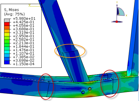
A job can now be created and the analysis run. To judge results, it makes sense to create an overlay plot of the global model and the submodel (Figure 14). This can be done via view -> overlay plot. In the regions where the node-based submodeling conditions is applied and displacements are prescribed (indicated with red ovals in Figure 14) the submodel is located at the same position as the global model, and stresses don’t match exactly. In the region where the surface-based submodeling condition is applied and surface traction is prescribed (indicated with orange oval in Figure 14) the displacement of the submodel is different from the displacement of the global model, but the stress forms a better match. This makes sense based on the prescribed end conditions. Because of this using surface-based modelling for stress results and node-based modelling for displacement results is most effective. Large displacements and rotations can only be taken into account with the node-based approach.

Figure 14: Overlay plot of global model and submodel.

As stated before, Abaqus does not check whether the submodel loads and boundary conditions that are applied make sense, it only applies them. Results from the submodel are limited by how well these conditions match reality. A too coarse global mesh can limit the accuracy of the boundary conditions. Also, the application of submodeling is based on Saint Venant’s principle: the solution in a local area of interest is not changed by end (far field) effects, as long as end loads remain statically equivalent. If the border of the submodel is too close to the area of interest, the applied conditions are not far field. The displacement or stress in the driving region of the global model would then change if a change in the region for which the submodel is made is applied (such as the switch from ties to a contact condition here). This change is not taken into account when using the submodeling technique. In the example shown here, consistency at the boundaries of the submodel may be improved if the submodel encompasses a larger region.

Summary

In summary, with submodeling you can use a global model to determine suitable loads and/or boundary conditions for a submodel and prescribe them. It is easy to apply. The main steps are creating a reference to the global model in the model attributes and applying appropriate submodel loads and/or boundary conditions. Because Abaqus does not perform any checks itself, it is import to ensure that the loads and boundary conditions were applied appropriately and that the assumption underlying the technique (boundary represents far-field loading) is valid by checking whether displacement (node-based submodeling) or stress (surface-based submodeling) is consistent in global model and submodel.