

Posted by Christine Obbink-Huizer
Categories
Abaqus 2022Table of contents
Abaqus 2022 is available. In this blog I will highlight some of the modifications and provide a list of other improvements so you can check them out yourself if the topic is of interest to you.
Writing about a new release is always challenging, because the list of new features is too long to describe everything in detail. We therefore need to pick topics to focus on. For this blog I chose features that solve a problem I have heard being discussed in the past, features that I expect are relevant to our customers in general, and features that can cause the software to behave unexpectedly. Since different users use different Abaqus features, the updates that are relevant to them will also differ. I therefore encourage you to read through the list at the end of this blog and find out more about the topics that interest you.
As in previous years, new functionality is not only added in the golden release, but also in hotfixes that become available throughout the year. Here I will mention functionality that became available since the last golden release.
The installation process is similar to that of Abaqus 2020, which is explained here.
Now let’s look at some new features and modifications:
Contact: Activate and Deactivate General Contact Interactions in Abaqus/Standard
Being able to activate and deactivate contact can come in handy, for example when there are multiple tools that do not all need to be accounted for in all steps. I recently learned – somewhat to my surprise - that this was not possible in general contact in Abaqus/Standard. Now, in Abaqus 2022 GA, this functionality is added. Contact inclusions and contact exclusions can be modified on a step level, to change the active contact region. If contact is removed in an region that is actively in contact, then the contact forces are stored and gradually removed during the step, as is done when contact pairs are deactivated in Abaqus/Standard. This new functionality makes general contact even more powerful and versatile.
Contact: Evolving Feature Edges On By Default Abaqus/Explicit
The edge-to-edge contact in Abaqus/Explicit can resolve contact situation that would otherwise go undetected. In the past, the edges considered by default were beam and truss elements as well as the perimeter edges of shells and membranes. During an analysis, feature edges may develop and become relevant for contact. When crumpling a piece of paper, for example, many edges develop that were not there at the start of the analysis. In the past, the Abaqus team has developed a method to find these newly developed edges and include them in the analysis. Now, performance improvements to this method make it only slightly slower than without including evolving feature edges, while the robustness and accuracy of the analysis is improved. For this reason, evolving feature edges are now included by default.
Scalar Valued Outputs Can Be Used As Field Variables
In Abaqus it is possible to let material properties depend on a field variable, where the field variable is a function of material point information. In the past, this was only possible using user subroutines (V)USDFLD and (V)GETVRM. Now it is possible to directly associate a field variable with a scalar valued output variable. This makes it easier and more user-friendly to use this capability.
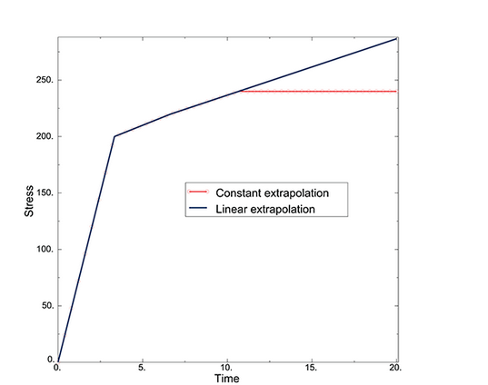
Linear Yield Stress Extrapolation Available
Plasticity data is defined in Abaqus using pairs of Yields stress and Equivalent Plastic Strain values. If the plastic strain exceeds the maximal value provided, then (by default) a constant extrapolation is used: there is no more hardening, the material behaves perfectly plastic and the plastic strain increases while the stress stays constant. This may lead to convergence issues, as the material is unstable. It is possible to add an additional data point, but that has drawbacks as well. For isotropic plasticity it is now possible to specify linear extrapolation, rather than constant extrapolation. In this case the slope between the last two data points is maintained outside the last data point provided. This option can be accessed using extrapolation=linear with the *plastic keyword via the keyword editor.
Hyperelasticity: Exactly Reproduce Test Results in Tension and Compression and Compression at the Same Time
The Valanis-Landel form of hyperelastic strain energy potential is now included in Abaqus. This model is similar to the Marlow model, in that no material fit is needed and instead the test data is reproduced. While the Marlow model is based on either tension or compression data when it is used with solids or shells, the Valanis-Landel model uses (and needs) both tension and compression data. The model can therefore produce a better fit.
Let’s take a look at an example, where I run a 1 element model for three different cases:
- The Marlow model, using only the part of the curve in compression
- The Marlow model, using only the part of the curve in tension
- The Valanis-Landel model using the entire curve
The result is as follows:
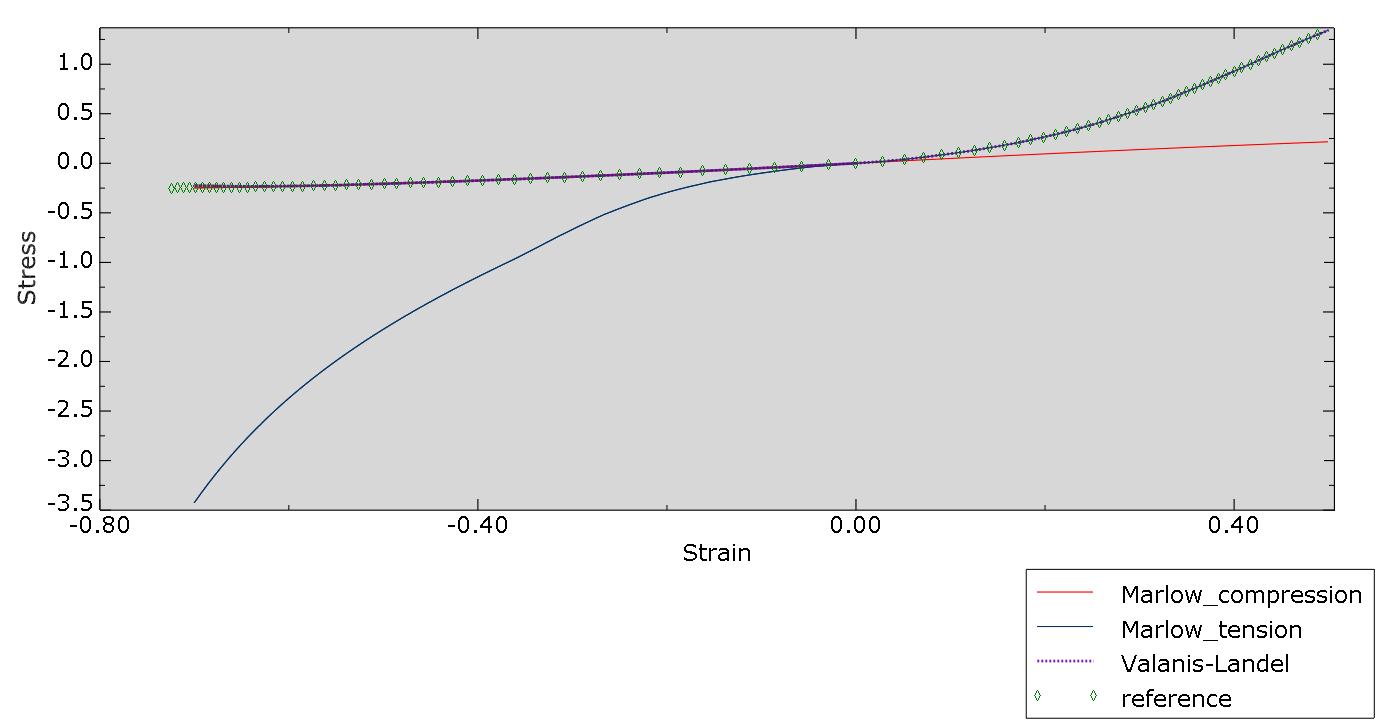
The Marlow model using only data in compression follows the compression part of the curve, but is too soft in tension. The Marlow model using only data in tension follows the tension part of the curve, but is too stiff in compression. The Valanis-Landel model matches the reference in both regimes.
The Valanis-Landel model is not available from Abaqus/CAE. You can use it e.g. by creating a Marlow model with uniaxial data ranging from compression to tension, and editing the keywords to change the hyperelastic definition into *Hyperelastic, valanis-landel.
One-Step Inverse Analysis
Abaqus now offers a procedure to estimate a blank from a formed product. In the first stages of design, this can be useful to estimate a blank size or trim line before the tooling is available.
To use this, a step with *one-step inverse procedure type is to be used. This is not available from Abaqus/CAE (yet), so manual keyword edits are required.
As a user, you need to provide the final geometry after forming/flanging. Only shell geometry is allowed and it is recommended to also provide nodal normals. Also specify a surface to represent the blank location. Define contact without allowing separation between the geometry and the blank location. Apply sufficient boundary conditions to avoid rigid body movements of the geometry. Abaqus will calculate the location of the nodes on the blank surface. It needs an initial estimate to start the algorithm. Therefore, you need to define:
*Initial Conditions, type=unfold coordinate.
This is to be done for each node. It cannot be done from Abaqus/CAE.
To get a feeling of this technique, I tried to run an example. At first I tried to unfold the final geometry from this blog. That did not converge with the effort I spent on it.
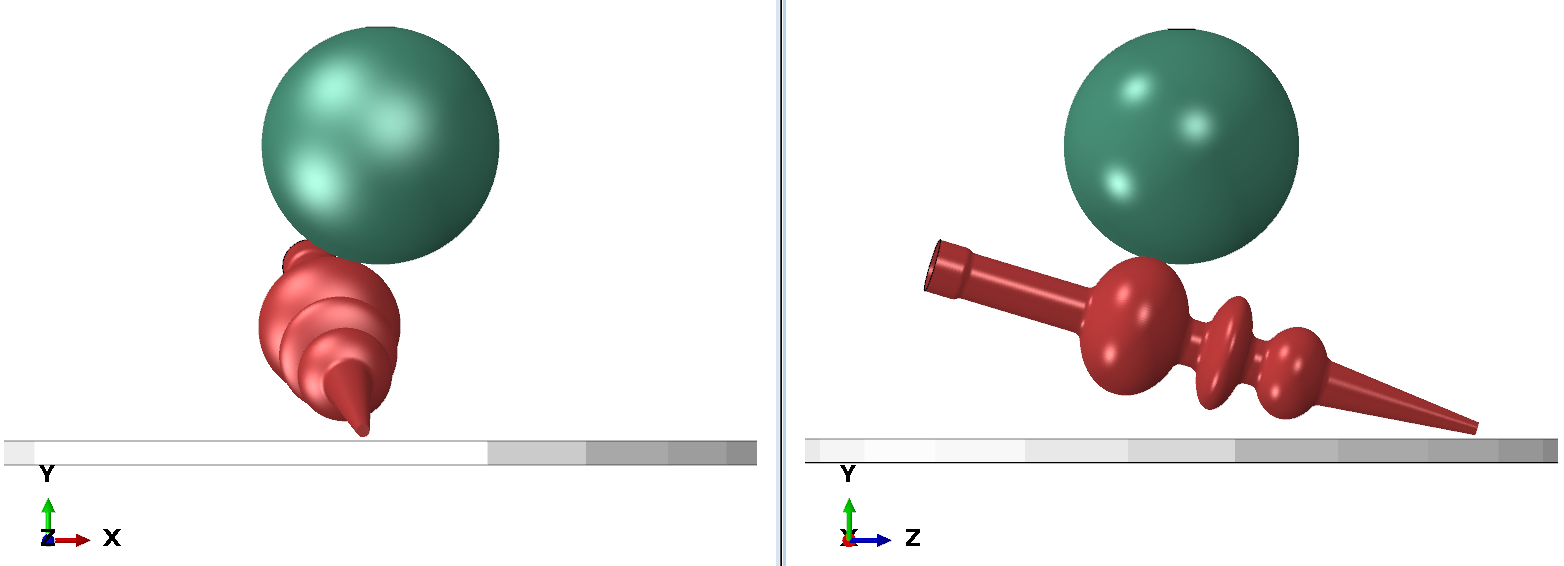
I then went to a simpler example. Here a curved sheet is unfolded to a flat blank. Only a thin slice is modelled. This is done with two blank locations, rotated 90 degrees with respect to each other.
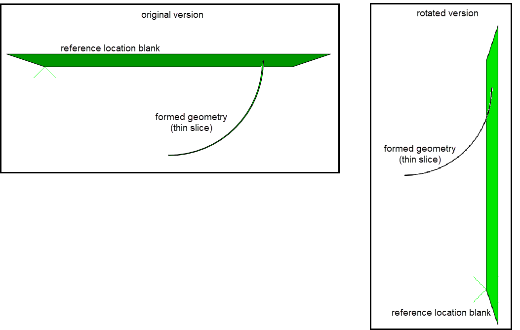
In this case the analyses ran. When the geometry is unfolded to a reference blank location on the top, there is an element with localized stains at the loose end. This is not the case when the geometry is unfolded to a vertical blank on the side. 
My simple tests indicated that though the functionality may be nice, it is not very easy to use. Especially obtaining the initial conditions can require some manipulation. In the test I did, results were not always obtained or intuitive. This can be my lack of knowledge on this topic, but at least is shows it is not a simple option where you click a few buttons and it always works.
Major Redesign of Substructure Functionality: All Previously Generated Substructures Need To Be Regenerated
In Abaqus 2022 a major redesign of the substructure functionality is introduced. The substructure .sim file is now the main file of the substructure database, and the substructure library file (.sup) is eliminated. Because of this, all previously generated substructures need to be regenerated. The overall workflow and results are not modified and the updated version of the functionality is set up in such a way that old input files are compatible. Please check the manual for more details.
List of Modifications
A complete overview of all modifications can be found in the Abaqus Release Notes section of the manual. This provides more detail than I do here. A Tech Talk on Abaqus 2022, also including some new features in 2022HF1 can be seen here.
General Enhancements and Modeling:
- Geometry and meshing enhancements in Abaqus/CAE:
- The ACIS version is upgraded from 2016 1.0.1 to 2021 1.0.0, allowing you to import or export ACIS 31 .sat files in Abaqus/CAE.
- You can select Cohesive Coupled Temperature-Displacement and Cohesive Coupled Temperature-Pore pressure element types in Abaqus/Standard.
- You can use linear kinematic conversion section control for Abaqus/Explicit.
- You can now select initial gap opening section control for Abaqus/Standard analyses.
- You can specify a local coordinate system when querying nodes, distances, and element face normals in Visualization module.
- Modeling enhancements in Abaqus/CAE:
- You can directly import CATIA V5 files as parts on the Linux platform.
- You can specify multiple directory locations in the Abaqus plugin_central_dir environment file parameter rather than just a single path. The standard path separator (a semicolon on Windows platforms and a colon on Linux platforms) must separate the directories.
- For the SOLIDWORKS Associative Interface for Abaqus/CAE:
- You can choose to export each body of a multibody part as a separate part in Abaqus/CAE.
- You can choose to maintain all region boundaries on parts exported to Abaqus/CAE.
- Abaqus/CAE considers the current assembly configuration in SOLIDWORKS when updating the model.
- In the composite layup editor, you can use an analytical field to specify the thickness of individual plies.
- For node-based submodeling, you can specify intersection only in the submodel boundary condition so that Abaqus ignores driven nodes found to lie outside the region of elements of the global model.
- Abaqus/Standard now supports shared memory parallel (SMP) analysis of large models with more than 16 million nodes.
- You can now define a distribution of local material directions (or fiber directions) for an anisotropic material. You can also use this feature to import local material direction results from an output database (.sim) file.
Analysis Procedures:
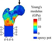
- Abaqus/Standard now offers an analysis capability aimed at simulating three-dimensional thermal-electrochemical processes in rechargeable battery cells based on an extended three-dimensional Porous Electrode Theory (PET) Newman model.
- The iterative linear equation solver is enhanced to support modeling features with Lagrange multipliers, such as hybrid elements, connector elements, distributing couplings, and hard contact.
- The performance of element output in linear analysis procedures is substantially improved.
- The AMS eigensolver is enhanced to support GPU acceleration on Windows platforms.
- You can now specify secondary base motion in local or global coordinate systems in modal transient and steady-state dynamic procedures.
- Element results output performance is substantially improved in response spectrum analysis procedures.
- You can generate data for flexible body dynamics in Simpack in a natural frequency extraction, which speeds up the process workflow.
- You can now perform a one-step inverse analysis in Abaqus/Standard to obtain the initial shape of a sheet metal part given its final (deformed) configuration and a reference blank surface to which the initial configuration must conform.
- You can now define a multiple nonlinear load case analysis to study the nonlinear responses of a structure subjected to distinct load histories consisting of one or more steps.
- The size of the models that Abaqus/Explicit can solve is increased significantly with this release.
Analysis Techniques:
- Several enhancements improve the usability of importing external fields from .sim files.
- Several enhancements improve the usability of import in Abaqus analyses:
- Abaqus now provides the capability to transfer nodal temperature and field variables from an Abaqus/Standard or Abaqus/Explicit analysis to an Abaqus/Standard or Abaqus/Explicit analysis when the material state is imported.
- You can now transfer model data and results of elements sets or part instances multiple times from an Abaqus/Standard analysis to an Abaqus/Standard analysis.
- An enhanced subcycling algorithm for interface handling for Abaqus/Standard to Abaqus/Explicit co-simulation is available.
- New naming conventions and a change for volume fraction thresholds are implemented in the special-purpose techniques for additive manufacturing.
- A pattern-based special-purpose technique is now available for powder bed–type additive manufacturing processes.
- You can now perform a sequentially coupled pore pressure–stress analysis that accounts for the effects of a known pore fluid pressure field.
- You can now include the temperature degree of freedom in a crack propagation analysis using the extended finite element method (XFEM).
- Elimination of the .sup file simplifies the substructure functionality, file management, and naming conventions, while ensuring backward compatibility in future releases.
- You can now use a single substructure generation procedure to generate a symmetric, an unsymmetric, or both a symmetric and unsymmetric instance of the stiffness and damping matrices, which produces results of improved quality at the usage level. You can also perform parametric studies by controlling the amount of unsymmetry in the substructure stiffness matrix at the usage level.
- Frequency-based substructures allow you to generate substructures that can exactly represent large models in direct steady-state dynamic analyses.
- The matrix check feature now allows you to modify the tolerances for checking substructure and generated matrices and to treat problems reported by the matrix check as errors. For substructures, the numerical condition is calculated and potentially insufficient retained node definitions are identified.
- Subassemblies: you can now specify interface nodes in the matrix generation procedure and use them to include generated matrices in the model in the matrix usage analysis.
- You can now use the cyclic symmetry analysis technique in explicit dynamic analyses to reduce simulation time and memory usage.
- The adaptive mesh refinement feature now allows you to improve the contact for Eulerian-Lagrangian contact interfaces.
- Fluid exchange based on the surfaces of failed elements is now available in Abaqus/Explicit to simulate fluid exchange through ruptured surfaces.
- The co-simulation approach where a Dymola-generated dynamic library (dymosim.dll) is linked to Abaqus is deprecated in favor of the FMI industry standard for system modeling.
- You can now define a milling geometric restriction for topology optimization.
- You can now select the PEMAG (Plastic Strain Magnitude) design response for sensitivity-based optimization types (shape, bead, sizing, and topology).
- You can select the MIMP (Mass Interpolation Material Penalization) parameter for the interpolation scheme.
- You can define SURF_TURN for sensitivity-based shape optimization.
- You can define the DRESP_GROUP_OPER_AGGREGATION group operator.
- You can select Check node group for a member size geometry restriction in a shape optimization. Several enhancements are available for optimization in Abaqus/CAE.
- Optimization enhancements are available for sizing and shape optimization tasks:
-
- You can now create a stress design responses (SIG_SENS_MISES) in a sizing optimization task.
- You can specify plane or cyclic symmetry with a nonsymmetric mesh in a shape optimization task.
-
- You can now request design responses and adjoint sensitivities for a three-dimensional linear model that includes inertia relief. You can also use various group operators for nodal design responses.
- You can now request design responses for implicit transient dynamic analyses and the corresponding adjoint sensitivities with respect to topology, sizing shell thickness, and sizing lattice design variables.
Materials:
- You can now use constant or linear extrapolation to evaluate the yield stress outside the specified data range.
- For elastic material behavior in Abaqus/Explicit, you can specify orthotropic elasticity in plane stress with different moduli in tension and compression.
- The multiscale material model now supports additional elements, which enhances the Abaqus capability to model fiber-reinforced composite laminates.
- You can now use Abaqus cure modeling capabilities to analyze the evolution of material properties and strains during curing processes.
- You can now model almost incompressible materials with the low-density foam model.
- You can now specify the time-temperature shift function of thermorheologically simple (TRS) materials in tabular form.
- The ply fabric damage initiation criterion with bilamina elasticity and shear plasticity is now available in Abaqus/Explicit for modeling and simulation of progressive damage of bidirectional fabric-reinforced composites. It is expected to replace the ABQ_PLY_FABRIC built-in user material previously available in Abaqus/Explicit.
- You can now turn rate-dependent yield and friction on and off within a step.
- You can now use the Valanis-Landel hyperelastic model to analyze material behavior.
- You can specify material properties as functions of material point state by introducing a field variable dependency and associating the field variable directly with a material point output variable.
- Band-limited damping in Abaqus/Explicit allows you to apply a desired uniform damping ratio over a specified frequency range.
- The modeling of short-fiber reinforced composites is improved.
- User control of transverse shear stiffness for shell elements when using user-defined material behavior is now available in Abaqus/Explicit.
- A local stabilized method involving pressure projections into the strain space is now available to eliminate spurious oscillations in a consolidation analysis with low permeability.
- The LaRC05 damage initiation criterion is now available in Abaqus/Standard, and the Hosford-Coulomb damage initiation criteria is now available in Abaqus/Standard and Abaqus/Explicit.
- You can now model metallurgical phase transformation during additive manufacturing processes or heat treatment processes.
- Several enhancements improve the usability of modeling materials in Abaqus/CAE:
- The Section Manager features a Material column to easily identify the materials associated with each section.
- You can create gap conductance, gap radiation, and gap convection material behaviors.
- For the creep model, you can specify the time type (total or creep) and the Anand, Darveaux, and double power laws.
- For the cap plasticity model, you can specify the time type (total or creep) and the power and time power laws.
- For the viscous model, you can specify the time type (total or creep) and the Anand, Darveaux, double power, power, and time power laws.
- For the Drucker-Prager creep model, you can specify the time type (total or creep) and the power and time power laws.
- For the plastic model, you can scale the yield stress and include the static recovery term with the nonlinear isotropic/kinematic hardening model.
- For the gap flow model, you can select the Bingham plastic or Herschel-Bulkley type to specify how you want to define the flow parameters.
- For the user material model, you can indicate that user subroutine VUMAT contains the effective modulus for an Abaqus/Explicit analysis and specify the hybrid formulation for hybrid elements in an Abaqus/Standard analysis.
Elements:
- New 3-DOF warping elements extend the meshed cross-section generation capability for composite beams such as those found in wind turbine rotor blades.
- You can now define full coupling between the six section strains and the six section forces and moments for a meshed beam general section and assign this section to element types B31 and B32.
- You can use a material definition to define the material properties of a general beam section. Channel-shaped and hat-shaped beam section types are now available in the standard beam cross-section library.
- Distortion control is now available for C3D10 elements in Abaqus/Explicit.
- You can now use distributions to specify layer thicknesses for composite solid elements and use wedge (triangular prism) elements with a composite solid section definition.
- You can use linear kinematic conversion to allow a simulation to continue for elements that are highly distorted due to large compressive forces.
Prescribed Conditions:
- You can now define a distributed nodal pressure load case analysis involving substructures in Abaqus/Standard to study the linear responses of a structure subjected to nonuniform pressure distributions.
- You can now define initial predefined field variables by importing field data from an output database (.sim) file.
Interactions and Constraints:
- Improved performance of general contact in Abaqus/Standard is available due to a new dynamic allocation strategy.
- Step-dependent contact activation and initialization and deactivation are available for general contact in Abaqus/Standard.
- To improve robustness, Abaqus/Standard considers the rotational degrees of freedom of cloud nodes in the rotational constraints of distributing couplings by default.
- Dynamic feature edge criteria are used when you specify that all feature edges for a contact surface should be activated.
- Several enhancements are introduced to improve performance and memory consumption for dynamic feature edge criteria.
- Automatic activation of edge-to-edge contact for all of the general contact domain dramatically improves the quality of the solution and usability of Abaqus/Explicit.
- "Softened" contact behavior is improved to allow nonzero pressure at zero overclosure and contact pressure as an exponential function of the clearance between surfaces in general contact in Abaqus/Explicit.
- Default "hard" contact behavior is improved to reduce penetrations when foam materials are involved in general contact in Abaqus/Explicit.
- The new dynamic memory management approach for solid erosion problems often results in dramatic memory reduction and 10% reduction in simulation run time.
- Several enhancements are available in Abaqus/CAE for defining general contact interactions.
- When you edit individual contact property assignments, you can directly select materials in addition to surfaces for the contact pairs. You can similarly select materials for surface thickness assignments, surface offset assignments, and surface feature edge criteria assignments.
- You can create new types of surface property assignments. For Abaqus/Standard you can create surface beam smoothing assignments and surface vertex criteria assignments. For Abaqus/Explicit you can create crush trigger assignments and surface friction assignments.
- You can activate the small-sliding tracking approach for interactions in Abaqus/Standard.
- For general contact in Abaqus/Standard, you can also
- specify secondary feature edge criteria for surface property assignments and
- control the smoothness of the surface-to-surface formulation upon sliding for specific interactions and control the edge-to-edge contact formulations.
- For general contact in Abaqus/Explicit, you can also
- specify secondary feature edge criteria and apply feature edge criteria statically or dynamically for surface property assignments and
- choose which sides of double-sided elements will be considered for node-to-face or Eulerian-Lagrangian contact with another surface for contact formulation.
- In Abaqus/CAE you can define additional geometric properties that will be accounted for in surface contact interactions.
- A terminology conversion from "master" to "main" and "slave" to "secondary" is implemented for Abaqus solvers and Abaqus/CAE.
Execution:
- The following enhancements are available for job execution:
- You can now select tokens or credits as a license type for DSLS SimUnit licensing.
- You can submit a job in Hybrid multiprocessing mode.
- The Abaqus adams translator performance is improved.
- You can now use the Abaqus make utility to create Abaqus user subroutines in individual dynamic link libraries or shared objects.
- Parallel execution of Abaqus/Explicit is now available in hybrid mode using a combination of MPI and threads.
- Several enhancements improve the usability for flexible body dynamics workflows involving Abaqus.
- Several enhancements improve the usability of the Abaqus from Nastran translator.
Output and Visualization:
- In modal analysis procedures, element output is now available for several connection types.
- New contact output variables are available in Abaqus/Explicit: CSHEARMAG (nodal frictional stress), CNAREA (nodal contact area) and CFRICWORK (nodal frictional work).
- Several enhancements are available for visualization in Abaqus/CAE:
- Channel and Hat beam profiles can now be rendered in the Visualization module of Abaqus/CAE.
- The Linked Viewport Manager provides options to Select All and Unselect All, which improves usability.
- Linked Viewport Manager option settings now persist between sessions.
- You can perform mathematical operations on X–Y data saved from field output.
- You can write local CSYS columns in the field output report.
- You can now request the Lode angle term output at an element material point.
- You can use the ODB Reducer/Builder plug-in (now included with Abaqus/CAE) to take portions of an Abaqus output database to create a new, smaller output database.
- In Abaqus/CAE you can now choose the position where selected field output values are written.
User Subroutines, Utilities, Plug-ins, and the Abaqus Scripting Interface:
- You can now use user subroutine VUGENS in Abaqus/Explicit to define the mechanical behavior of a shell section.
- You can now define your own element design response based on either the stress tensor or the plastic strain tensor of the element integration points.
- You can now define the strain energy potential of an isotropic hyperelastic material in terms of deviatoric principal stretches and the elastic volume ratio.
- User subroutines FRIC_COEF and VFRIC_COEF are enhanced to allow friction coefficient dependence on additional contact slip variables.
- You can now access physical constants defined in an input file from any Abaqus/Standard user subroutine.

TECHNIA Simulation provides top tier FEA, Non-linear, and Advanced Simulation Software, Training, and Consultancy. Our dedicated team of more than 65 Simulation experts across 16 countries advise and support your innovation with a wealth of specialist knowledge and experience.
About TECHNIA- Related news and articles straight to your inbox
- Hints, tips & how-tos
- Thought leadership articles

Helping you find the information you’re looking for. Discover webinars, events, FAQ's, case studies and tutorials.
VIEW HUB