
Posted by Nikolaos Mavrodontis
Table of contents
In this post we will be showing an exemplary analysis with Abaqus Standard. This analysis will incorporate a coupled thermal-stress problem of a cylindrical shell (e.g. a pipe enclosing a high temperature fluid used in a factory). This pipe will be connected to a metallic expansion joint that will have the purpose of undertaking the thermal extension of the pipe. The purpose of the coupled analysis will be to demonstrate the mapping of result values via the predefined field option.
Coupling the Thermal and Structural Domains
Abaqus offers many modelling options for coupling thermal and structural domains in an analysis.
Typically two methods can be used:
1)Combining the thermal loading and induced displacements in a single analysis, with use of coupled temperature-displacement elements (SAX2T, S8RT,C3D20RT etc.)
2) Modelling the thermal load on the structure in a first analysis and then mapping that thermal load (via Nodal Temperatures, NT) on a subsequent stress analysis.
In this blog the 2nd option will be demonstrated. If all effects of different types of loads are to be considered (axial pressure, hoop pressure, thermal load etc), in many occasions the 1st method might be a more feasible option.
Modelling Assumptions
- The model will incorporate a cylindrical shell structure, a pipe enclosing a high temperature fluid. For this analysis, only a thermal load is considered due to the temperature difference on both sides (inner and outer) of the pipe.The pipe will be considered stiff enough to not deform circumferentially under fluid pressure (only axial translations will be allowed in for the static analysis).
- For the analysis a cylindrical shell model (complete cylinder) has been used for the sake of clarity. It is advised however that axisymmetry (or single elements even with appropriate boundary conditions) is used as often as possible to reduce runtimes.
-For analysis 1, a steady state heat transfer analysis will be considered.
-For analysis 2, a static general analysis will be considered.
-For all analyses, S8R5 elements were used.
-The materials of the expansion joint and the fluid pipe are linear elastic. For real life situations, the materials are not necessarily the same. This varies per application, but whenever non-metallic expansion joints are used in low pressure applications, these are usually much more flexible (rubberlike materials) than their connecting parts.
-Stress results are given in Mpa. Displacement results are given in mm.
For this investigation, two analyses will be run. First a heat transfer analysis, on a pipe segment with inner temperature of 200 degs Celsius and outside(ambient) temperature of 10 degs Celsius. This temperature difference will cause expansion of the pipe in the circumferential as well as in the axial direction. Consequently a stress analysis will be run, wherein the temperatures from the previous heat transfer procedure will be mapped on the mesh in order to estimate the induced stresses and displacements caused due to the thermal load. This analysis can provide input for the design of the expansion joint.
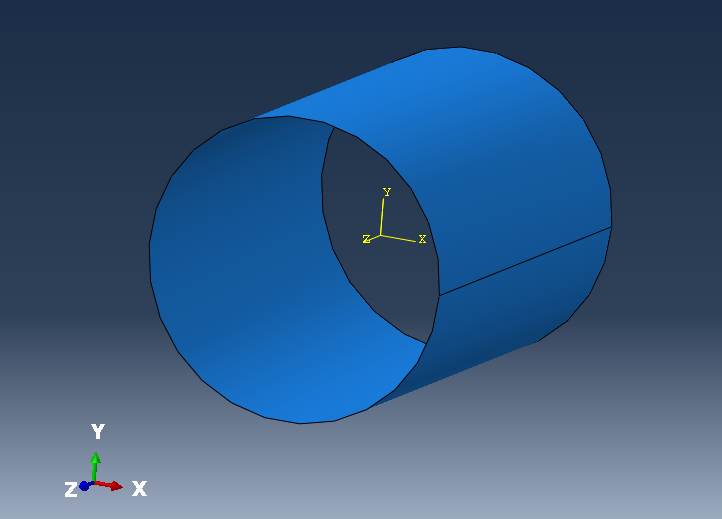
The fluid pipe geometry is given in Figure 1.
-3.png?width=640&name=figure%201%20(pipe%20assembly)-3.png "Abaqus pipe assembly")
Figure 1: Fluid Pipe Geometry.
Heat Transfer Analysis
For the steady state heat transfer analysis, the two temperature boundary conditions are applied on all nodes on the appropriate degrees of freedom. This is shown in Figure 2.
-Apr-21-2022-03-26-48-03-PM.png?width=640&name=figure%202%20(heat_transfer_Bcs)-Apr-21-2022-03-26-48-03-PM.png "Abaqus heat transfer boundary conditions")
Figure 2: Heat transfer boundary conditions.
Figure 3 shows the pipe temperature reached at the end of the heat transfer step (10 degrees Celsius).

Figure 3: Heat transfer end step temperature conditions.
Static General Analysis
For the static general analysis , the extracted node temperature field from the heat transfer analysis is given as input as a predefined field. In order to do that, the user must give the path to the respectful heat transfer odb. This is shown in Figure 4.
-Apr-21-2022-03-26-42-19-PM.png?width=640&name=figure%203%20(temperature_pre_field_input)-Apr-21-2022-03-26-42-19-PM.png "Abaqus temperature_pre_field_input")
Figure 4: Temperature predefined field.
In order to also discover the benefits of expansion joints , a simplified expansion joint model will b included in the static analysis. The connection details and some terms are given in Figure 5.
As was mentioned in the modelling assumptions, the pipe will be allowed to extend only in the axial direction. This axial extension of the fluid pipe will be undertaken by the expansion joint. This expansion joint will be connected to a rigid connection (e.g. concrete wall) on its free side (Z-displacement =0).
.png?width=640&name=figure%206%20(expansion%20joint%20detail).png "Abaqus expansion joint detail")
Figure 5: Joint and assembly details.
The stress results of the static general analysis and the axial displacements of the assembly are given in Figures 6 and 7,8 respectively.

Figure 6: Stresses on the assembly.

Figure 7: Axial displacements of the assembly.

Figure 8: Axisymmetry view cut of the assembly.
The video below shows the deformation of the expansion joint due to the axial extension of the pipe under thermal loading.
Conclusions
The coupled thermal-stress analysis capabilities of Abaqus were demonstrated in this post. The main focus was to demonstrate the predefined field option that Abaqus incorporates.
When the two analyses (heat transfer and static general) are run sequentially the predefined field can be used to map relevant results as input for the second analysis.
This technique can be extended to other domains (e.g. cooling down of metal parts in combination with mass diffusion of certain elements). In cases where loads of different type are to be investigated together with thermal loads, it might be more practical to use method 1 for an analysis.
Additionally the coupling rules (loose, strict etc.) can be further assigned by the user, by changing relevant solver settings.
When these type of analyses are run and shell elements are used, it is best to use quadratic shell elements that can provide results closer to the analytical solutions.
Solid elements and continuum shell elements can be used as well but with proper mesh generation rules (e.g. more than one element in thickness direction).


TECHNIA Simulation provides top tier FEA, Non-linear, and Advanced Simulation Software, Training, and Consultancy. Our dedicated team of more than 65 Simulation experts across 16 countries advise and support your innovation with a wealth of specialist knowledge and experience.
About TECHNIA- Related news and articles straight to your inbox
- Hints, tips & how-tos
- Thought leadership articles

Helping you find the information you’re looking for. Discover webinars, events, FAQ's, case studies and tutorials.
VIEW HUB