
Posted by Nikolaos Mavrodontis
Table of contents
In this blog post, we will be discussing about some of the most commonly used hardening laws that are available within Abaqus, and can be deployed whenever a metal’s plastic (inelastic) behavior and the nature of the applied load (monotonic, cyclic) becomes relevant in the modeling.
In this post, we will not be discussing about the elastic perfectly plastic material law (no hardening-bilinear) nor about the multilinear kinematic hardening law.
Unit cube (area of each face equal to 1mm^2) tests have been set up, meshed with a single continuum element (C3D8R), that will showcase with more clarity, the effects of using a different hardening law on the produced stress-strain paths.
The type of loading will be of uniaxial cyclic nature (tension-compression), and it will be stress based, implemented as a pressure load acting on the cube’s face (YX plane face).
Loads and Boundary Conditions
Figure 1 shows a detail of the loads and boundary conditions acting on the unit cube . In order to achieve cube deformations that trully correspond to uniaxial loading conditions, appropriate symmetry conditions have been applied in the 3 faces (not visible on the viewport). In terms of the input load amplitude, a simple ramp-up to a maximum tensile stress and a ramp down to zero stress, followed by a simple ramp up to a maximum compressive stress (not considering signs) and a ramp down to zero stress. This can be described as one loading cycle. The tensile and compressive maximums will be the same (proportional) but also different (non-proportional), based on the case at hand. Load tables will be provided per case studied, to properly track the input pressure load.
-3.png?width=1634&name=Figure%201(loads%20and%20BCs)-3.png)
Figure 1: Pressure load vectors, amplitude definition detail and boundary conditions of unit cube model.
Material Properties
Figure 2 shows the elastic and plastic tab definition of the used material. The hardening law implemented in the plastic tab of Figure 2, is isotropic hardening. The elastic tab will be common for all the different cases that will be investigated
The plastic tab input will vary based on the hardening law showcased. What will be kept common in the plastic tab, for all load cases, will be the first row of data, corresponding to the “virgin” yield stress(σ0) at zero plastic strain. Subsequent row data, will depend on the used hardening law and its calibration against test data.
-2.png?width=1053&name=Figure%202(elastic-plastic-properties)-2.png)
Figure 2: Exemplary material properties used in the model (elastic properties-left, isotropic hardening properties-right).
For the purposes of this blog post, the hardening laws have already been calibrated against relevant test data. More information on how to calibrate the various kinematic hardening laws against test data can be found in the abaqus documentation, using the link below.
Yield Surface
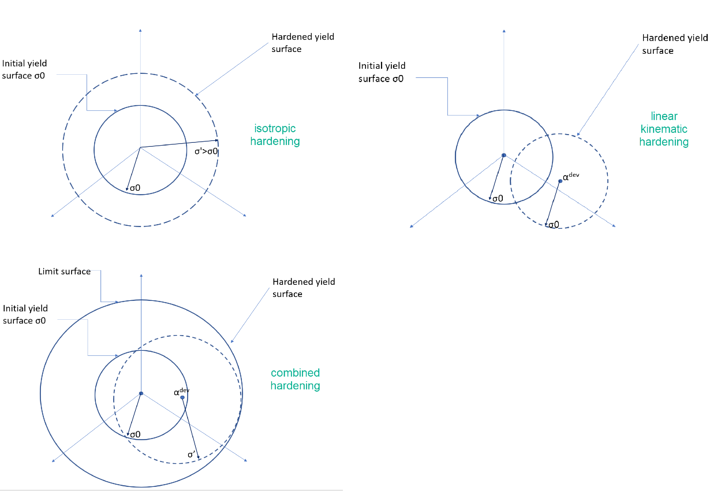
The yield surface that will be used for all load cases/hardening laws used will be the von Mises yield surface. The von Mises yield surface is graphically represented in 3d stress space below, in figure 3.
v3-1-1.png?width=711&name=Figure%203(yield%20surfaces)v3-1-1.png)
Figure 3: original yield surfaces and evolution of yield surfaces per hardening law.
Whenever a material point under stress, is within the yield surface, it remains fully elastic. Whenever a material point is at or outside of the boundaries of the yield surface, it is yielding (deforming inelastically).
Based on the hardening law chosen, the center of the yield surface can stay fixed in stress space, but its radius can increase while more inelastic strain is accumulated. This is called isotropic hardening. Alternatively, the center of the yield surface can move in space, but not grow (constant radius) while more inelastic stain is accumulated. This is called linear kinematic hardening.
Lastly, the von mises yield surface can move in space and grow upon accumulating more plasticity on a material point. This is called combined nonlinear isotropic/kinematic hardening law and it is the most intricate hardening law, available within the software.
These three hardening laws will be demonstrated, under different stress-based loading conditions, and their usage limitations will be explained with respect to modelling certain behaviors that real life metals show under certain loading conditions.
Load Cases
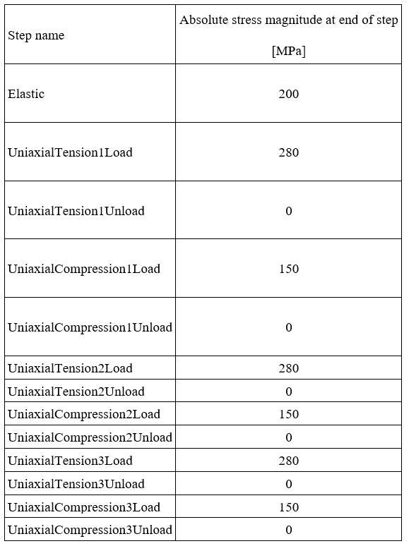
Below you can find a summary of the absolute stress magnitudes , at the end of each load step per load case. Those provided values, will help trace the produced stress-strain paths more easily, during post processing.
Case 1
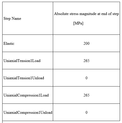
Load table 1 is shown below. The stress levels at the end of each step (t=1) are given below in MPa.
Table 1: Case 1 Absolute stress values at end of each step (t=1).
Case 2
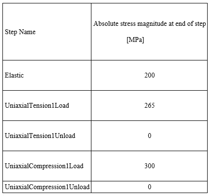
Table 2: Case 2 Absolute stress values at end of each step (t=1).
Case 3
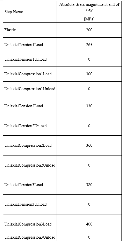
For case 3, three loading cycles will be implemented, essentially, transitioning to cyclic loading (compared to Cases 1,2).
Table 3: Case 3 Absolute stress values at end of each step (t=1).
Case 4-combined Hardening Specific Load Case
This load case is specific to the combined hardening law. This case will consist of 9 load cycles in total, where the directional stresses (tension, compresison) will be strongly non proportional in this case. The tensile loading will be more severe than the compressive loading, and this will demonstate the ratchetting phenomenon (more information in later sections), observed under non proportional cyclic loading.
Table 4, only shows the first 3 loading cycles. 6 more loading cycles (total of 9) will be simulated, having the same stress levels as those shown in Table 4.
Table 4: Case 4-combined hardening law specific: Absolute stress values at end of each step (t=1)
Results
The results of the single element will be assessed in terms of plotting the stress (S33) in MPa vs logarithmic strain (LE33). Those results were extracted from the (only) integration point of the C3D8R element.
Isotropic Hardening
Case 1
Case 1 concerns a single load cycle (tension-compression) while making use of the isotropic hardening law. As shown in table 1, a first loading step will load the unit cube in uniaxial tension up to its first yield stress (virgin yield stress σ0). Then the tensile load will be increased up to 265 MPa and then reversed, down to -265 MPa of uniaxial compression, and back to zero load input.
_v2-3.png?width=711&name=Figure%204(1loadcycle_isotropic_max265)_v2-3.png)
Figure 4: Load case 1 (Table 1) - isotropic hardening-stress-strain paths.
Figure 4 shows the S33 stress vs logarithmic strain (L33) results as extracted at the integration point of the single C3D8R element.
We can see that the first knee point is made at the end of step 1 (elastic). Then the material hardens up to the maximum tensile stress (265 MPa). Then we start to unload/reverse loading direction, all the way down to -265 MPa. This is the “new” yield point that the isotropic hardening law will predict. Since we do not apply a compressive load lower than -265 (e.g. -280), there will be no additional hardening. The material will then unload elastically back to a zero-stress state, following the exact same path of the loading in compression (end of Uniaxialcompression1Load= end of niaxialcompression1Unload).
To better comprehend the yield stress prediction of the isotropic hardening model, let us provide a definition of isotropic hardening behavior:
Isotropic hardening behavior presumes that yielding of material in unloading (load reversal), occurs when the stress range is changed by twice the value of the highest stress reached prior to unloading (Δς=2σ’ in figure 4).
This is what we are essentially seeing in figure 4, also indicated by the green line to the right. The compressive yield stress (-265 MPa) predicted by this hardening law, will be equal to twice the range of the max stress experienced prior to the load reversal (265 MPa).
Case 2
The loading information of case 2 is shown in Table 2. The difference compared to case 1, is that now, higher compressive loads will be reached (-300 MPa) in order to activate isotropic hardening also for the compressive cycle.
v2-3.png?width=1622&name=Figure%205(case_2_1loadcycle_isotropic)v2-3.png)
Figure 5: Load case 2 (Table 2) - isotropic hardening-stress-strain paths.
From figure 5 it is evident now, that the compressive loading (endofUniaxialCompression1Load) and unloading paths (endofUniaxialCompression1Unload) do not coincide, as hardening took place for the compressive cycle. Still the predicted knee point (first yield) in compression, was equal to -265 MPa, as this is inherent to the isotropic hardening law.
Case 3
Case 3 includes 3 loading cycles in total, as shown in Table 3. Also, the absolute (excluding signs) maximum stress magnitude at the end of every step, will be greater than the previous one, essentially modelling hardening in every half cycle.
-3.png?width=1651&name=Figure%206(case_3_3loadcycles_isotropic)-3.png)
Figure 6: Load case 3 (Table 3) - isotropic hardening-stress-strain paths.
The extracted results are shown in figure 6. We can now see that all loading/unloading paths are separated from one another, as hardening takes place in every step. You can notice that the predicted yielding upon load reversal (knee points, B, D,F), takes place at a stress level that is changed by twice the value of the highest stress reached prior to the load reversal (A,C,E).
What happens, is that the hardened yield surface stays fixed in space, but its radius grows. This is evident by comparing the lengths of AB, CD, EF. We can see that the length (or half length) of EF is greater than CD and the length of CD is greater than the first loading cycle (AB). This effect on the stress-strain path, corresponds to the growth of the yield surface, on the left-hand side photo of Figure 3.
Linear Kinematic Hardening
Case 1
The same cases as shown for isotropic hardening, will be now set up while making use of the linear kinematic hardening law, available in Abaqus.
The loading conditions of case 1, with linear kinematic hardening are identical to those shown in Table 1.
v2-1.png?width=711&name=Figure%207(case_1_1loadcycle_linear_kinematic)v2-1.png)
Figure 7: Load case 1 (Table 1) -linear kinematic hardening-stress-strain paths.
Figure 7 show the S33 stress versus the L33 strain graph of case 1.
Similarly to what we did with the isotropic hardening, we will establish a definition of the linear kinematic hardening, to better understand the yield stress prediction given by this hardening law:
Kinematic hardening predicts that yielding upon load reversal, occurs when the stress change from the unloading point (σ’ in Figure 7) is twice the monotonic (virgin) yield stress (Δσ=2σ0). Those characteristics are demonstrated in Figure 7.
The predicted yield stress in compression (kneepoint =-135 MPa) has a stress difference equal to 2*200 ΜPa from the preceding unloading point in tension (σ’=265 MPa).
Case 2
The loading definitions of this case have already been provided in Table 2.
.png?width=1716&name=Figure%208(case_2_1loadcycle_linear_kinematic).png)
Figure 8: Load case 2 (Table 2) -linear kinematic hardening-stress-strain paths.
The respective results of case 2 with the linear kinematic hardening law are shown in figure 8. Those are quite comparable to case 1, as the only difference here is that a higher compressive stress level is achieved, and naturally more plastic strain in compression is accumulated (shifting the strain path more towards compression, compared to case 1).
Case 3
The loading definitions of this case have already been provided in Table 3. The respective results are given in Figure 9 for 3 loading cycles.
-3.png?width=1715&name=Figure%209(case_3_3loadcycles_lin_kin)-3.png)
Figure 9: Load case 3 (Table 3) -linear kinematic hardening-stress-strain paths.
The linear kinematic hardening yield stress prediction is respected in Figure 9 for all loading cycles.
Essentially the stress range here (Δσ) stays constant here, regardless of the additional hardening taking place per cycle. This is since the yield stress prediction will always take place at a stress level equal to 2σ0 which is constant.
The effect that this has, is that the length of Δσ does not increase upon every load reversal(so the size of the yield surface stays the same) but the yield surface moves in space (as shown in Figure 3), as the material accumulates more plasticity (the stress-strain loops become wider on the horizontal axis).
Combined (Non Linear) Hardening
Case 1
For case 1, the combined nonlinear isotropic/kinematic hardening law will be used in Abaqus. The same loading conditions of table 1 will be applied here.
The stress-strain results are given in Figure 10. Also plotted, are the case 1 results from the isotropic hardening (dashed green line) and the linear kinematic hardening models (solid red line)
.-Apr-21-2022-03-57-41-10-PM.png?width=1639&name=Figure%2010(1loadcycle_combined)-Apr-21-2022-03-57-41-10-PM.png)
Figure 10: Load case 1 (Table 1) - combined hardening-stress-strain paths
The yield stress(knee point) prediction upon load reversal, for both the linear kinematic and the combined hardening laws, is the same (indicated by blue circles above), but the hardening modulus (defines the slope of the yellow line above) of the combined law , resembles the one from the isotropic hardening law, for the simple case of 1 load cycle.
Case 2
The stress-strain results for case 2 are given in Figure 11. Also plotted, are the case 2 results from the isotropic hardening (dashed green line) and the linear kinematic hardening models (solid red line).
-1.png?width=1526&name=Figure%2011(case2_combined)-1.png)
Figure 11: Load case 2 (Table 2) -combined hardening-stress-strain paths.
Case 3
The stress-strain results for case 3 are given in Figure 12. Also plotted, are the case 2 results from the isotropic hardening (dashed green line) and the linear kinematic hardening models (solid red line).
The nonlinear stress strain behavior predicted by the combined hardening law is more evident in Figure 12.
-1.png?width=1844&name=Figure%2012(case3_combined)-1.png)
Figure 12: Load case 3 (Table 3) -combined hardening-stress-strain paths.
Case 4
This load case was specific to the combined hardening law. The results from all 9 load cycles are given in Figure 13.
-Apr-21-2022-03-57-10-18-PM.png?width=1646&name=Figure%2013(ratchet_combined)-Apr-21-2022-03-57-10-18-PM.png)
Figure 13: Load case 4 (Table 4) -linear kinematic hardening-stress-strain paths.
It can be seen that since the maximum stress values are tensile (280 MPa) , and in the compressive regime, lower stress values are applied (150 MPa), we have a mean stress that is tensile. The effect that this has, is that the yield surface moves in space towards tensile(positive) strains. Essentially hysteresis loops are formed on every load cycle, meaning that more plastic strain is accumulated on every load cycle.
If those hysteresis loops ,moving to the right, in Figure 13, coincide with one another, after a number of loading cycles (after some initial plastic strain has been accumulated), this is a favorable situation, called shakedown. Essentially, the material point accumulates (initial) plasticity upon every new load cycle, but after a certain number of load cycles, it shows an elastic behavior.
On the other hand, if the hysteresis loops continue moving to the right, with every new load cycle (as shown in Figure 13) this is called ratcheting or cycle dependent creep. This is not a favorable situation at all. With every new cycle more plasticity is accumulated and this behavior continues for all load cycles. The structure will essentially fail.
Limitations of the Hardening Laws
The isotropic hardening law should be used when the induced strains are unidirectional ( no load reversal). So in practice , it is not an accurate enough model for cyclic loading . As seen in physical testing, when hardening takes place in tension, and then the loading is reversed ( compression), the actual yield strength in compression will be lower than its tensile analogous. This is called the Bauschinger effect.
Essentially the material point will yield prematurely in compression (compared to the equivalent tensile yield stress value). The isotropic hardening law, only predicts symmetric yield stress levels (Figure 4), and therefore cannot capture the Bauschinger effect.
The linear kinematic model is a simple model that gives only a first approximation of the behavior of metals subjected to cyclic loading(such as the Bauschinger effect). The nonlinear isotropic/kinematic hardening model can provide more accurate results in many cases involving cyclic loading, but it still has the following limitations:
-
The isotropic hardening is the same at all strain ranges. Physical observations, however, indicate that the amount of isotropic hardening depends on the magnitude of the strain range. Furthermore, if the specimen is cycled at two different strain ranges, one followed by the other, the deformation in the first cycle affects the isotropic hardening in the second cycle. Thus, the model is only a coarse approximation of actual cyclic behavior. It should be calibrated to the expected size of the strain cycles of importance in the application.
-
The same cyclic hardening behavior is predicted for proportional and nonproportional load cycles. Physical observations indicate that the cyclic hardening behavior of materials subjected to nonproportional loading may be very different from uniaxial behavior at a similar strain amplitude.
The non linear combined hardening law is the most accurate buiit in model in Abaqus, for describing material response under cyclic loading. Its limitations are demonstrated in the following links.
Simple proportional and nonproportional cyclic tests
Uniaxial ratchetting under tension and compression


TECHNIA Simulation provides top tier FEA, Non-linear, and Advanced Simulation Software, Training, and Consultancy. Our dedicated team of more than 65 Simulation experts across 16 countries advise and support your innovation with a wealth of specialist knowledge and experience.
About TECHNIA- Related news and articles straight to your inbox
- Hints, tips & how-tos
- Thought leadership articles

Helping you find the information you’re looking for. Discover webinars, events, FAQ's, case studies and tutorials.
VIEW HUB