
Posted by Christine Obbink-Huizer
Categories
isightTable of contents
Isight is probably best known for its capabilities to do optimization. However, this is not the only thing Isight can do. Isight also includes the option to create an approximation, for example. With this, a mathematical equation is fitted to the actual behaviour of one or more components. This approximation can then be used in other Isight models, so it is not necessary to run the actual component(s) each time. This can save a lot of time. In this blog, I’ll show how to make an approximation in Isight and what results data is available.
Example Abaqus model: Sinterklaas’ staff
Keeping in mind the time of the year, we’ll take a look at Sinterklaas’ staff. A model is made in Abaqus (Figure 1), by extruding a circle along a path.
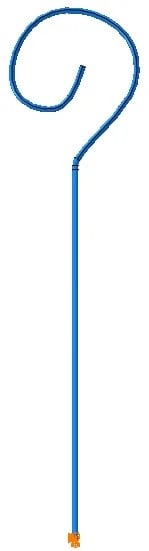
Figure 1: Geometry of Sinterklaas' staff
The resulting solid is converted into a shell using the create shell: from solid option. The staff is fixed in all directions at the bottom, where it is on the floor, and it is loaded with gravitational loading. We will approximate the relationship between shell thickness and the radius of the staff cross-section (inputs) and the mass and maximal displacement of the staff (output). To make it easier to find the parameter referring to the radius of the staff in Isight, a parameter is created for this in the relevant sketch (figure 2).
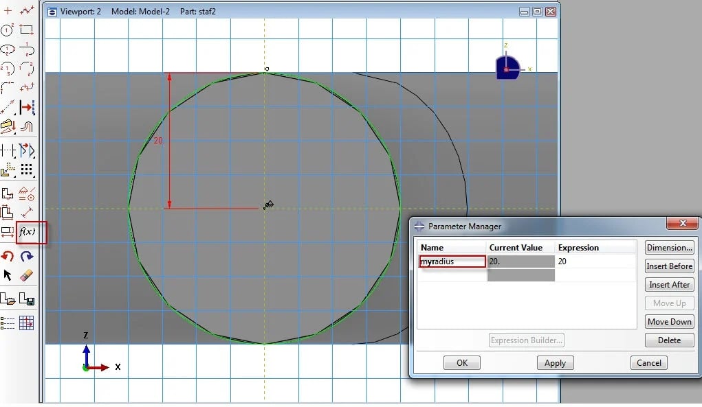
Figure 2: Creating a parameter for the radius in Abaqus
Mass output and displacement field output are requested. Other default outputs are switched off, to limit the size of the output databases. Once the model is set-up, a job is created an run. This is done both to check the model for mistakes, and to have an example .odb available. The .cae is saved and Abaqus is closed.
Isight: Abaqus component
The Isight design gateway is started with a default simflow and an Abaqus component is dragged on it (figure 3).
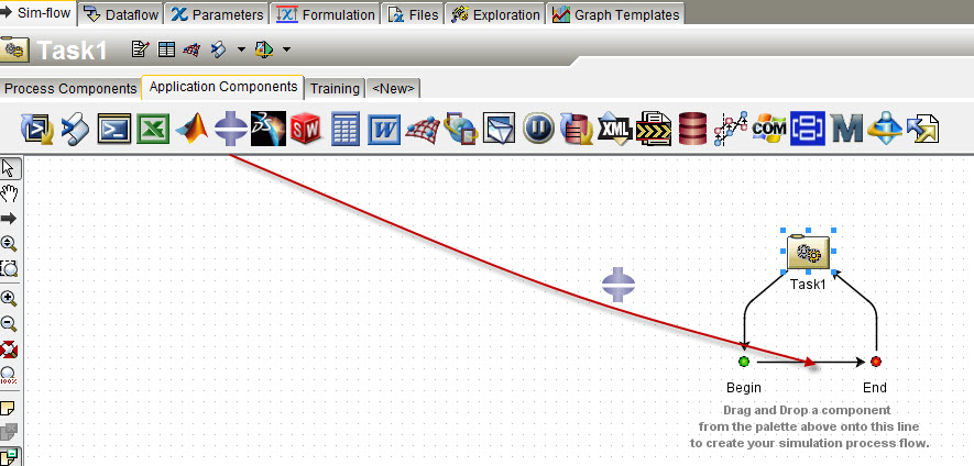
Figure 3: Abaqus component is dragged on Isight simflow
The Abaqus component is opened for editing, and the .cae is selected. Isight can work with both .cae’s and .inp files. Inp files do not contain geometrical parameters, they only contain the mesh. Because a geometrical parameter (the radius of the staff) will be modified, in this case the .cae needs to be selected. After the file is read, the available parameters are displayed and the relevant can be selected. The parameter name that was defined in the Abaqus sketch is recognizable (Figure 4).
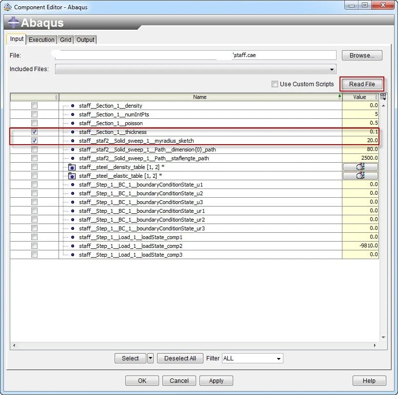
Figure 4: Selecting the relevant input parameters in the Abaqus component editor
The execution options are checked. In the output tab, the odb is selected and read, similar to the .cae file. Here the Mass and maximal displacement magnitude are selected. With this, the Abaqus component is set up and can be used in a simflow.
Isight: Approximation
An approximation can be made on a component, by right-clicking the component and selecting: approximations (figure 5).
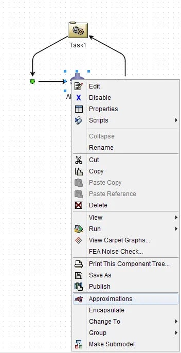
Figure 5: Creating an approximation by right-clicking the component
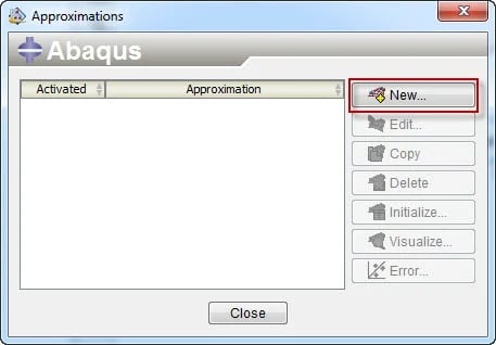
Several approximations can be created on the same component, though only one can be used at run time. For this example, a new approximation is created (figure 6).
Approximation technique
Several approximation techniques are available within Isight. The technique determines which mathematical equations are used to describe the relationship between inputs and outputs of the component. The available options are response surface model, orthogonal polynomial model, RBF model and Kriging model. A description of each technique is available in the selection screen, to help make this choice.
The response surface model is based on a polynomial fit. It is the most commonly used technique. Obviously making a polynomial fit will work best if the function to be fit is (similar to) a polynomial. This is the case for smooth functions if the volume of the design space is small enough. The minimum number of points required to make the fit increases with the number of input variable. Therefore, the response surface model works best for well-behaved functions with a small number of variables. Results from the approximation do not necessarily match the data points it is fitted on.
The technique of Radial Basis Functions (RBF) is based on neural networks. Elliptical basis functions (EBF) are a variant to this that requires more initialization time, but is better a capturing directional effects. Results from the approximation exactly match the data points it is fitted on, so noise is not filtered out. The approximation improves as more data points are included.
Kriging assumes autocorrelation: that the value of the function at a point is correlated to values nearby. Different autocorrelation functions are available. This model captures complex local nonlinear shapes. It works best with uniformly distributed data points and performs reasonably well with a limited number of data points.
In this case, we will start with a response surface model. If the errors using this model are deemed small enough, it will not be necessary to move towards a more complex model (Figure 7).
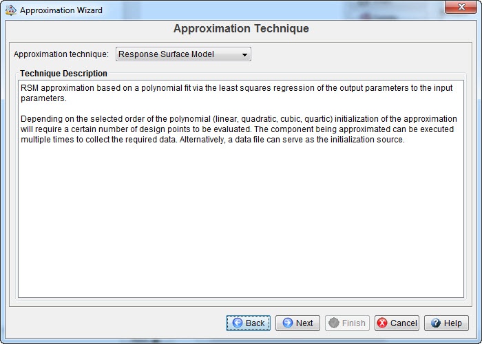
Figure 7: Selecting an approximation technique. A description is given to aid the selection.
All previously defined inputs and outputs are used for the approximation. A quadratic polynomial will be used.
Obtaining sampling points
Besides specifying a technique, it is also necessary to specify the data points on which the fit will be based. There are three ways of doing this: by letting Isight generate random points, by specifying a DOE matrix or by providing a data file. This data file should contain the values of inputs and outputs. It can be obtained from previously run analyses or from experimental results. This options does not require the component to be run in order to make the approximation. For the other two options the component does need to be run to obtain the data. With random points, the points used for the fit are random, as the name indicates. When using a DOE, the points are sampled using a specified technique. In this case the optimal latin hypercube method is selected, with 25 points (figure 8).
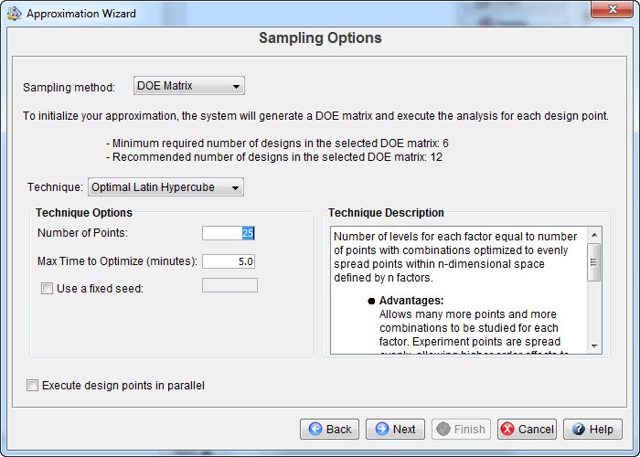
Figure 8: Selecting the sampling method. As for the approximation technique, a description of each DOE techniques is available to aid in the selection.
We need to decide the range within which the values can be modified, in this case the range will be from -50% of the base line value to + 50% of the base line value (Figure 9).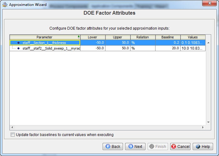
Figure 9: Selecting the ranges of the inputs
It is important to think about the region for which the approximation will be made, as an accurate fit can more easily be made in a smaller region, but results outside the approximated range will be unreliable. With this information, the DOE design matrix can be generated: Isight can create a list of input parameter combinations that will be used to fit the model.
Error analysis
Before an approximation can be used, we need to know how accurate it is. Within the approximation wizard, two different error analysis methods can be selected: either using a separate data set, or using cross-validation. If a separate data set is used, the original data will be used to create a fit and the results from this fit will be compared to the actual results, as given in the separate data set. Usually an approximation is made when it is time consuming or difficult to obtain data. Therefore obtaining additional data for error analysis may not be preferred. Cross-validation does not require additional data. Instead, it removes one point from the main data set, creates a new fit and compares results of this fit to the output of the removed point. This does not require additional data, but it does require additional model fits to be made. The amount of points to be removed for cross-validation can be specified. Here we will use all 2.
Approximation improvement
Isight has the option to generate additional data points if the error of the initial fit is too large. This will not be used now.
Initialization
When the approximation is defined, the fit needs to be made. This is called initialization. Isight will ask whether the initialization is to be done directly when the approximation wizard is finished. When clicking yes, the design points will be executed. This takes some time. The results can be seen as they are calculated. When the initialization is finished, Isight shows the calculated coefficients and provides options for error analysis and visualization (Figure 10).
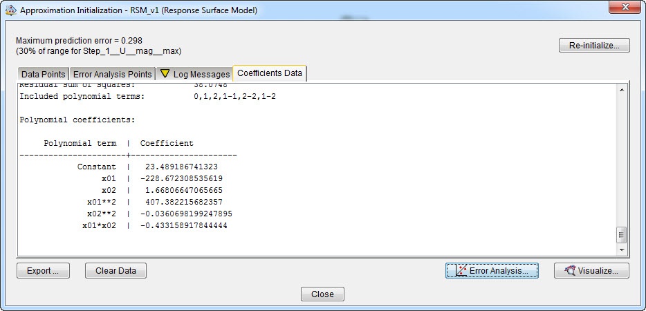
Figure 10: approximation results
Results
Error analysis
The error analysis tab shows the actual versus predicted output for each of the test points analyzed. Different error types can be calculated: the average, maximum, and root mean square. For these outputs, smaller values correspond to a better fit. An acceptance level can be filled in. If this level is not reached for a certain output, the corresponding graph becomes red (figure 11).
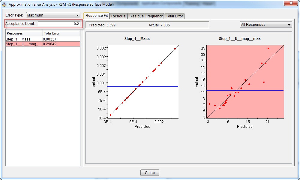
Figure 11: Error analysis for quadratic response surface model
This makes it easy to see where the approximation model is not good enough. In this case, we see that the mass is predicted nicely, while the error on the displacement magnitude is bigger. We may obtain better results by increasing the amount of polynomial terms, or using a different technique.
Visualisation
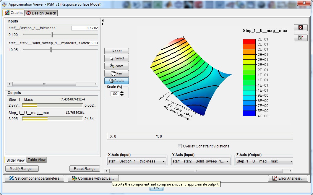
Of course we would like to know what the relationship between our input and output parameters looks like. 2D graphs (Figure 12), 3D graphs (Figure 13) and contour graphs (Figure 14) are available to get an idea of this. The 3D graphs can be rotated.
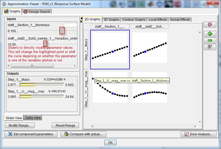
Figure 12: 2D graphs for mass or maximal displacement magnitude vs shell thickness or staff radius. As indicated in the image, the sliders allow direct visualization of the influence of changing parameters.

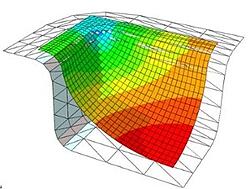
Figure 13: 3D graph for the maximal displacement magnitude vs shell thickness and staff radius.
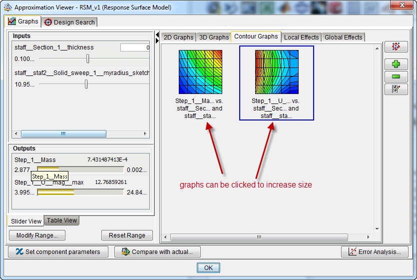
Figure 14: Contour graphs for mass vs shell thickness and staff radius and maximal displacement magnitude vs shell thickness and staff radius.
Most of these graphs are created by default, they are directly available when selecting the appropriate tab. If not, it is easy to create an additional graph, by simply selecting the desired inputs and outputs.
In this case, the mass increases with both section thickness and staff radius, as expected. The displacement reduces with increasing section thickness, while there is a maximum displacement at an intermediate staff radius.
Modifying the approximation technique
For the displacement, the maximal error in the current model is almost 30% of the range of the parameter and the average error is more than 7%. This is quite high. A different approximation technique may provide a better fit. When we edit the approximation and use polynomials up to fourth order terms, it is not necessary to recalculate the sampling points: Isight suggests using the previously calculated ones. With this model, the error is smaller (figure 15) and the contours of the displacement look different (figure 16).
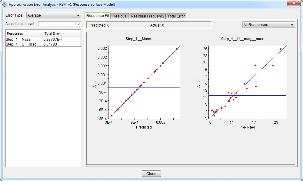
Figure 15: Error analysis for response surface model with terms up to and including fourth order. The average error is now below 5%, compared to more than 7% for the second order model.
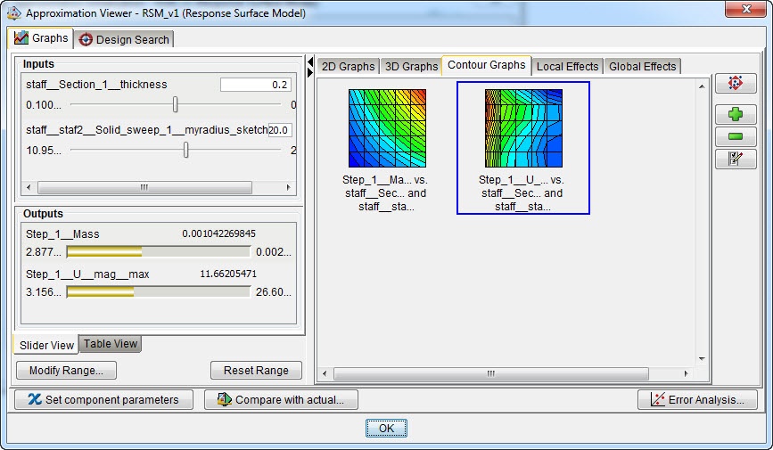
Figure 16: Visualized approximation for response surface model with terms up to and including fourth order.
With the EBF technique, the fit is better (figure 17) and the contours of the displacement are again somewhat different (figure 18).
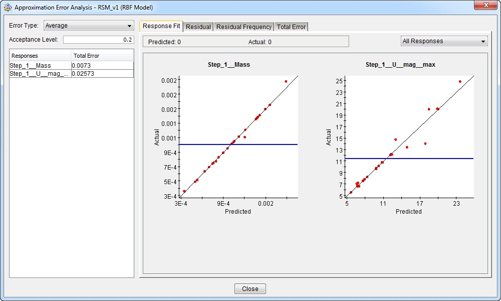
Figure 17: Error analysis for elliptical basis functions model. The average error is now around 2.5%, compared to 5% for the fourth order RSM and 7% for the second order RSM model.
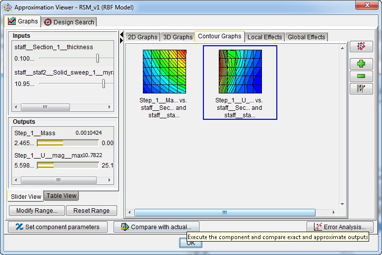
Figure 18: Visualized approximation for response surface model with elliptical basis functions.
Searching a design
Within the approximation viewer, it is possible to search for a design using the design search tab. A range is specified for the design variables. By default this is the range used to fit the model, so that the approximation is valid in the range used. Constraints can be specified as well, in this case the mass should not be more than 1 kg. Finally, objectives are given, in this case that the maximal displacement is to be minimized. By clicking ‘search’ Isight tries to find the point that matches the objective and constraints given (Figure 19).
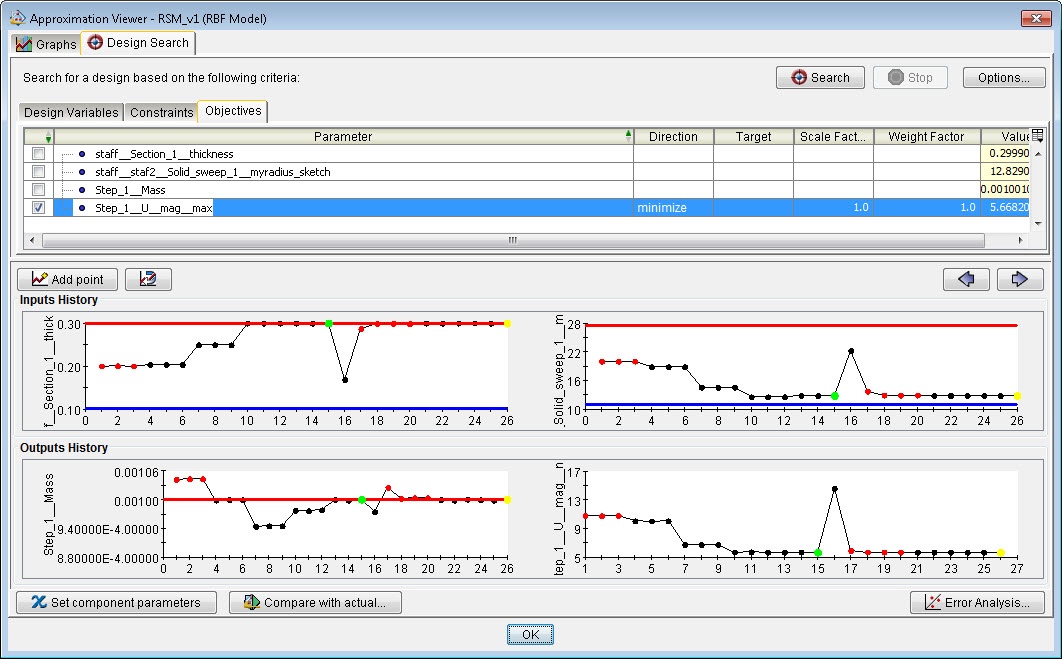
Figure 19: Using the design search option, to find a design matching certain objectives and constraints
Conclusion
This blog gave an example op setting up an approximation in Isight and showed some of the results and visualization options that er available. Once the approximation is deemed satisfactory it can activated to be used in other sim flows. Instead of running the actual code (the Abaqus model in this case) the description in the approximation will be used, which is much faster. This makes is more reasonable to use the (approximation of the) component in cases where it needs to be run often.

TECHNIA Simulation provides top tier FEA, Non-linear, and Advanced Simulation Software, Training, and Consultancy. Our dedicated team of more than 65 Simulation experts across 16 countries advise and support your innovation with a wealth of specialist knowledge and experience.
About TECHNIA- Related news and articles straight to your inbox
- Hints, tips & how-tos
- Thought leadership articles

Helping you find the information you’re looking for. Discover webinars, events, FAQ's, case studies and tutorials.
VIEW HUB