
Posted by Nikolaos Mavrodontis
Table of contents
In this blog post, we will be demonstrating the material calibration capabilities of the Material Calibration App, available through the 3DEXPERIENCE Platform. Two different materials will be calibrated against input test data, in order to attain their material parameters, necessary for finite element analyses. The resulting material models will include hyperelastic and linear/non-linear viscoelastic behavior.
This post will also highlight some of the exclusive material calibration capabilities of the Material Calibration App.
Calibration
Calibration is an enabling technology. It allows the user to develop a mathematical model that closely matches an observed behavior. In the case of material calibration, we are looking for the optimum values that design variables of material laws (e.g. E-modulus, Mooney-Rivlin material coefficients) must have, in order to attain the best-fit to the observed behavior (e.g. the stress-strain relationship derived in testing).
Calibration can be set-up in various ways, from manual trial and error on a single software, to involving more software to automate the process. You can read a nice blog on this from Christine, here.
Optimization Problem
The basic questions of the optimization problem are the following:
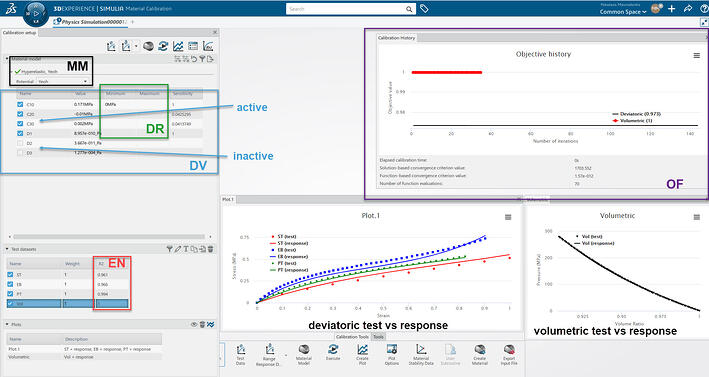
- What can we change? The design variables (DV). Modulus of elasticity, hyperelasticity material model coefficients etc.
- By how much? Minimum and maximum ranges (DR) need to be defined.
- What is the design variable relationship to the response? The material model (MM) used (e.g. σ=Ε*ε) in the calibration.
- How well does the response correlate to the test data? We assess specific error measures (EN) and plots showing the correlation between optimized material law and test data.
- What improvements are desired? To minimize the objective function (OF). This is shown in a graphical form , and is dependent on the type of EN currently used (among other things). So if for instance the R2 error norm is used (yes the same one used in curve fitting in Excel), the objective function is maximized (1).
- Since we are interested in finding the optimum solution (e.g. the optimum material coefficient values of our model in order to match the behavior) during calibration, the how-to achieve that, depends on the optimization algorithm used. You can read more about the optimization algorithms available in the app, here.
Figure 1 below, shows an impression of the app's interface, and also annotates the components used in the optimization process, as mentioned above.

Figure 1: Material calibration app user interface and components.
Execution Modes
This app, offers highly automated material calibration capabilities and can be run in two execution modes:
- Analytical mode: Uses analytical forms (equations) of many material constitutive laws (e.g., linear elastic , Johnson-Cook plasticity, hyperelasticity+Mullins effect) during the calibration process. This mode is ideal for calibration (e.g. finding the optimum solution), as analytical material models can be optimized faster, than numerical ones.
- Numerical mode: Uses Abaqus components (unit cube models with material subroutines) and tries to match (as closely as possible) the stress/strain state observed in testing. Subsequently, the material law is attained. The execution process (optimization) in this mode, usually takes longer.
Why are both modes available then? The numerical mode allows access to a larger material law library, already implemented in Abaqus. However, more analytical models are currently being implemented, and will be available in upcoming releases.
Material Calibration Examples
Test Data Input and Manipulation
For test data input, the app supports both Excel spreadsheets and text based files (*.csv,*.txt). Additionally the user can perform input data cleanup operations, such as zero shift, smooth and decimate (data point reduction).
Below, you can see a video from the test data input in the app for the exemplary rubber material, for three deformation modes, including volumetric test data.
ST-Simple Tension
EB- Equi-Biaxial mode
PT- Planar Tension
Vol-Volumetric data
Video 1: Rubber material test data input in the material calibration app.
Additional comments Video 1
- The stress-strain data points are always plotted as nominal stress vs nominal strain, for the material models within the app. Keep that in mind in case you want to model metal plasticity, as your test input data then, will be valid up to the ultimate strength and not further (in the necking region, where strains become non uniform). You should therefore remove data points past this ultimate strength point, as those will not be valid.
- If the user would still like to model metal plasticity, then the material will need to be calibrated against a finite element mesh. This functionality will soon be available in the material calibration app.
For optimization purposes, it is beneficial to have just the right amount of input data, to reflect the material behavior in testing. Having data with high sampling frequencies (a lot of data points), can impact the optimization runtimes.
The video below, shows an example of decimating (reducing) the number of volumetric test data points, for the material calibration. The original test data set included 245 data points of pressure vs volumetric ratio. The decimated dataset included 100 data points while still accurately capturing the rubber's volumetric behavior.
Video 2: Rubber material volumetric test data decimation in the material calibration app.
Rubber Material Xalibration (Hyperelastic)
Video 3 below, shows the material calibration process for the rubber material in the app. A hyperelastic material model including volumetric data was used. In the end a 2nd order polynomial was used as the optimized material law, as this achieved the best deviatoric and volumetric response to the test data (observed behavior). Specifically the R2 measure achieved was 0.993 and 1 , for the deviatoric and volumetric responses respectively. An impression of this, is shown in Figure 2.
Video 3: Rubber material calibration process in the material calibration app.
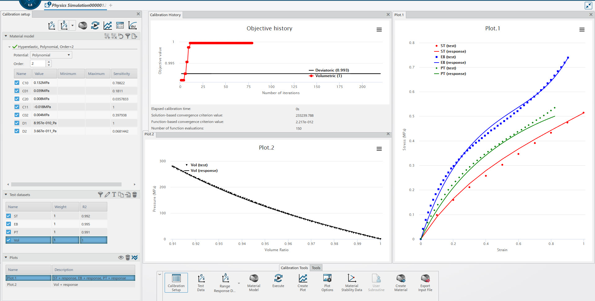
Figure 2: Material calibration app user interface and components.
Additional Comments Video 3, Figure 2
- The initial values of material coefficients (C10,C01,...) will generally influence the convergence and runtimes of the optimization algorithms. This is why if specific information is known a priori (e.g. the value of C10), this information should be provided as input from the user, before calibrating.
- The "calculate sensitivities" option is a quick way to assess the influence of changing a design variable, on the calibrated material law. When the calculated sensitivity of a design variable is really small , the user can deactivate this design variable and re-calibrate. If the calibrated response is not affected by the removed design variable (you can assess the response visually and from the error norm R2) , then the respective design variable should stay deactivated. Fewer design variables means faster runtimes for the optimization. This difference in runtimes might not be distinguishable when running in analytical mode(as those models are really fast anyway) but it will be distinguishable when running in numerical mode.
Enforcing Material Stability
The material calibration app offers material stability information, similar to the "evaluate material" printed output in Abaqus. A nice feature of the material calibration app, allows for enforcing material stability during calibration. This means that if a resulting material model is unstable, within (or outside of) the strain range of interest, then the user can enforce material stability within predefined strain ranges. The optimized material law will eventually be a stable one.
The video below, shows a calibration example (revisiting Video 3), starting from an unstable material law, and resulting in a stable one, upon enforcing material stability.
Video 4: Enforcing material stability during calibration in the material calibration app.
Figure 3 shows the material evaluation comparison, for the initially unstable material law (top) and the resulting stable one (below).
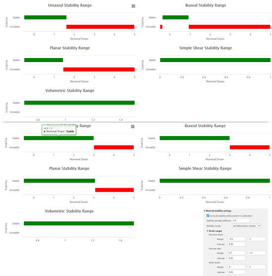
Figure 3: Material stability evaluation, unstable (top) vs stable (bottom) -enforcing material stability during calibration.
Additional Comments Video 4, Figure 3
- In our example case, the provided input test data ranges result in an a priori stable material law. The enforce material stability feature is used to simply extend the stability of the resulting mathematical model onto greater strain ranges.
- A stable material law as described just above, can be used for testing purposes or to assist convergence in f.e. analyses. For instance if there is a local hotspot forcing the stresses/strains to be larger than the stability limits of the used material law, the material law can be substituted with an enforced stable one, to assist convergence.
- It is important to remember that attaining material stability outside of tested ranges (observed behavior), will not give accurate results in an fe analysis, since no corresponding test data will be available for the correlation.
- However the enforce material stability feature, might be beneficial for a tested material that is unstable within the ranges of interest.
Plastic Material Calibration (Hyperelastic + Viscoelastic)
Linear Viscoelasticity
A hyperelastic plus viscoelastic material model behavior (Prony series) can be calibrated in Abaqus. For this exemplary input of plastic material, we have used a neo - Hookean material model and 4 stress relaxation test data, each one at a different strain rate (for calibrating the viscoelastic part).
Video 5, shows the calibration process. The analytical execution mode is used (fast) and the mean square error is used as an error norm. Minimization of the OF is intended.Different optimization algorithms are explored.
Video 5: Calibrating plastic material with Prony series viscoelasticity in the material calibration app.
Figure 4 below, shows the end result of the calibration, using Prony series and linear viscoelasticity.
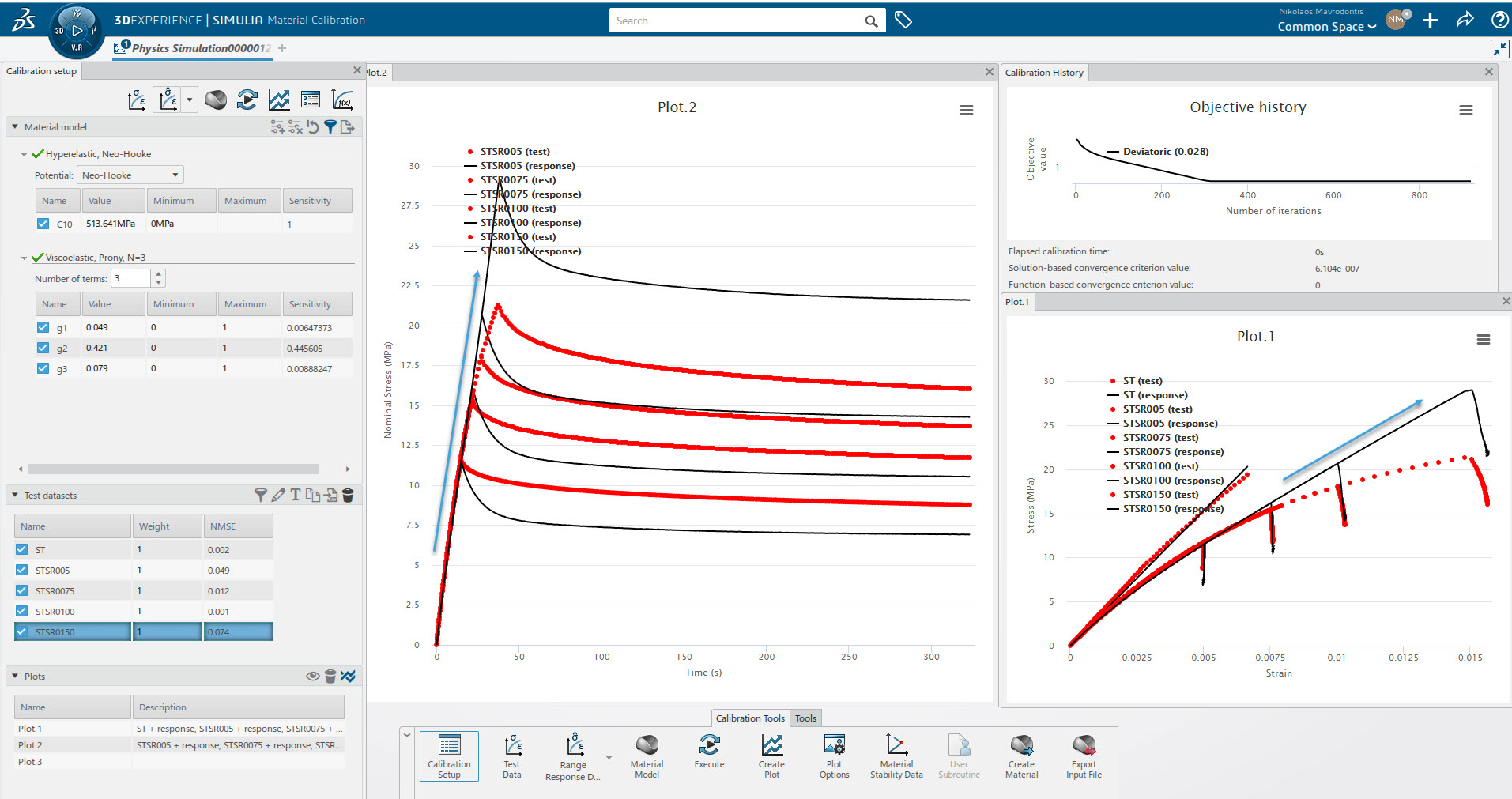
Figure 4: Calibrated plastic material with Prony series viscoelasticity in the material calibration app.
For this particular plastic, it can be seen that the viscoelastic behavior is non-linear. The predicted response with Prony series, is relatively poor, due to the limitations of the linear viscoelasticity model. This is evident in the NMSE error measure.
Non-Linear Viscoelasticity (Parallel Rheological Framework- PRF)
For this calibration run , we substitute the Prony series model (Figure 4) with the PRF for the viscoelastic component of the material.
The PRF material model is supported only in numerical mode execution. Therefore we expect the runtimes to be greater than what has been demonstrated so far.
Video 6: Calibrating plastic material with PRF non-linear viscoelasticity in the material calibration app
Figure 5 below, shows the end result of the calibration, using Prony series and linear viscoelasticity.
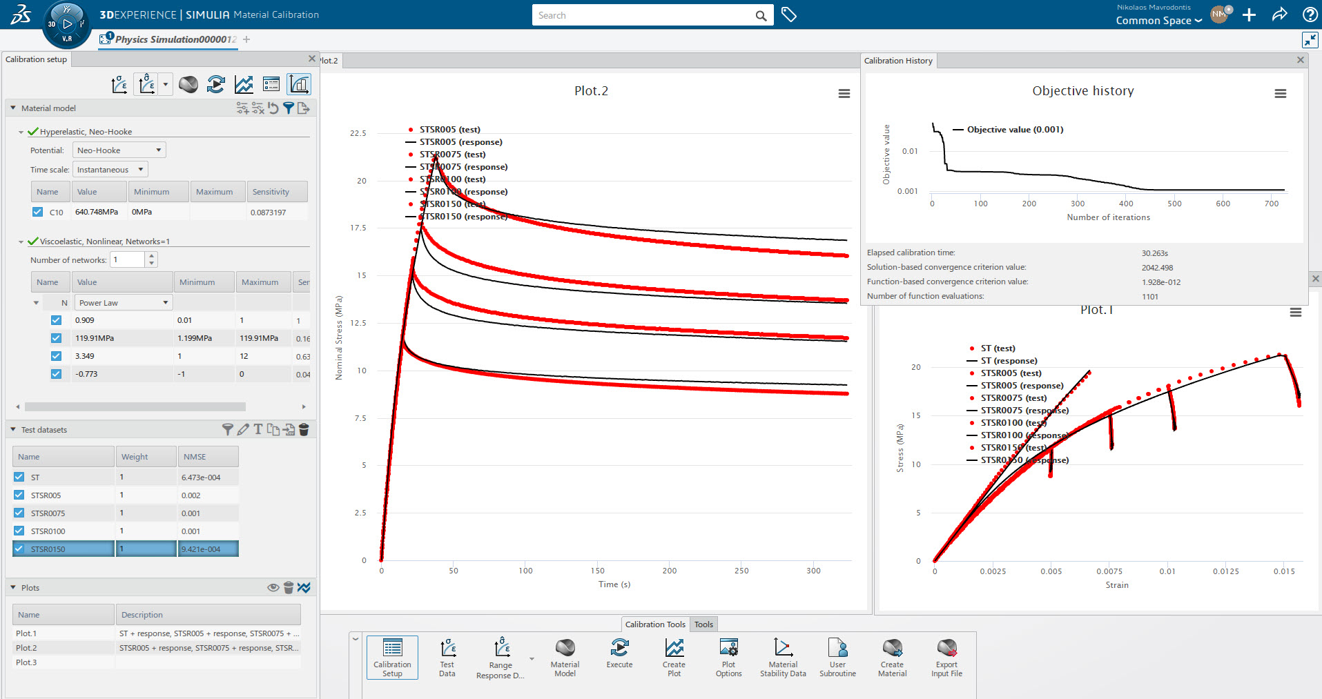
Figure 5: Calibrated plastic material with PRF non-linear viscoelasticity in the material calibration app
By comparing EN of Figures 4 and 6, and also visually, the improvement in the captured viscoelastic response with the PRF, is evident, for the optimized material.
Then we can simply export the material model as *.inp , or save it as a material model in the 3DEXPERIENCE Platform, to be used further.
Concluding Remarks
- New material models in analytical execution mode (fast) and more calibration options are being implemented for the material calibration app.
- This app offers the possibility to simultaneously calibrate hyperelastic plus viscoelastic material behavior, from a family of strain rate curves, stress relaxation tests etc. This accounts for both linear (Prony series) and non-linear viscoelasticity (PRF). This functionality is currently not available in Abaqus.
References
The input test data used, was provided to Simulia by Axel Products.


TECHNIA Simulation provides top tier FEA, Non-linear, and Advanced Simulation Software, Training, and Consultancy. Our dedicated team of more than 65 Simulation experts across 16 countries advise and support your innovation with a wealth of specialist knowledge and experience.
About TECHNIA- Related news and articles straight to your inbox
- Hints, tips & how-tos
- Thought leadership articles

Helping you find the information you’re looking for. Discover webinars, events, FAQ's, case studies and tutorials.
VIEW HUB