
Posted by Nikolaos Mavrodontis
Table of contents
Concrete Frame Under Earthquake Loading Using Abaqus
In this post, we will be demonstrating the setup of an earthquake analysis. The structure to be investigated will be a concrete frame. The earthquake input signal will have the form of an acceleration time history (lateral accelerations vs time) with a signal frequency of 100 Hz.
Soil structure interaction will also be included with use of concrete foundations embedded (tied) on the surrounding soil segment.
The concrete foundations will support the concrete frame that will undergo a certain motion under earthquake loading. The acceleration time history will be applied on the nodes of the soil at a lower level.
Parts
The concrete frame that constitutes the structure under earthquake can be seen below. It has been modelled with beam elements, with a rectangular profile (0.5 m x 0.5 m). Typical concrete linear elastic properties have been assigned. This structure is shown in Figure 1.
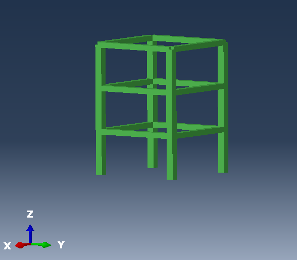
Figure 1: concrete frame.
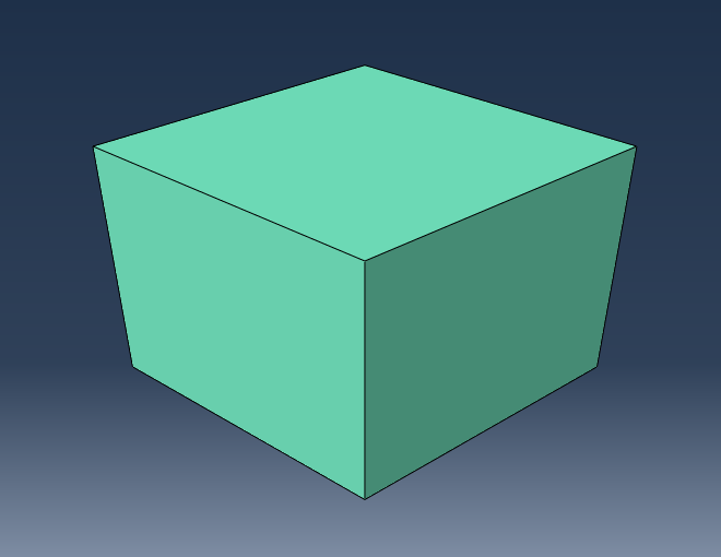
At the lower ends of the 4 concrete beams of the structure, 4 concrete blocks are tied, serving the purpose of the structure’s foundations. One of the 4 concrete foundation blocks is seen below. The material properties for the foundations are the same as for the structure. Figure 2: shows one of the foundation blocks.
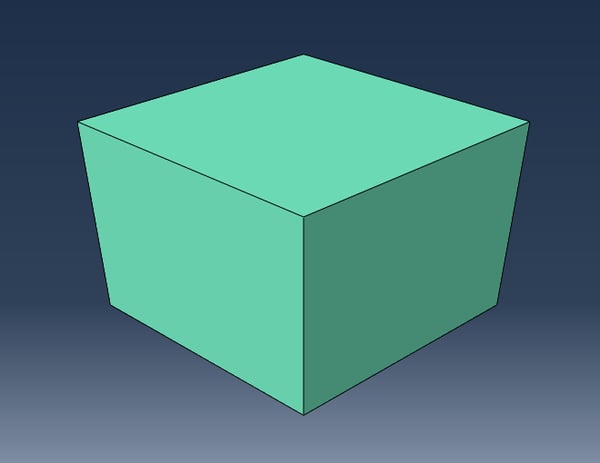
Figure 2: foundation block.
An in-between soil segment has also been created. It serves the purpose of allowing mesh refinement around the location of the structure and foundation blocks. This soil segment has the same soil properties (linear elastic) as the larger soil block.
A detail of the connection between concrete and soil segment is seen in Figure 3.
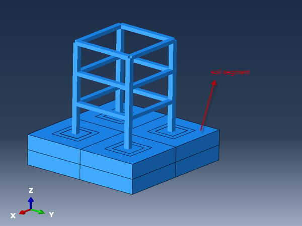
Figure 3: detail of frame-foundation-soil segment.
A large soil block has been created and typical linear elastic soil properties have been assigned to it.
The soil block can be seen below. On its top, an extruded cut has been created so that the soil segment can be connected.
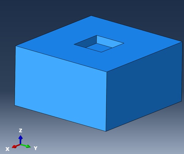
Figure 4: detail of frame-foundation-soil segment.
Assembly
The assembly of the various parts can be seen below.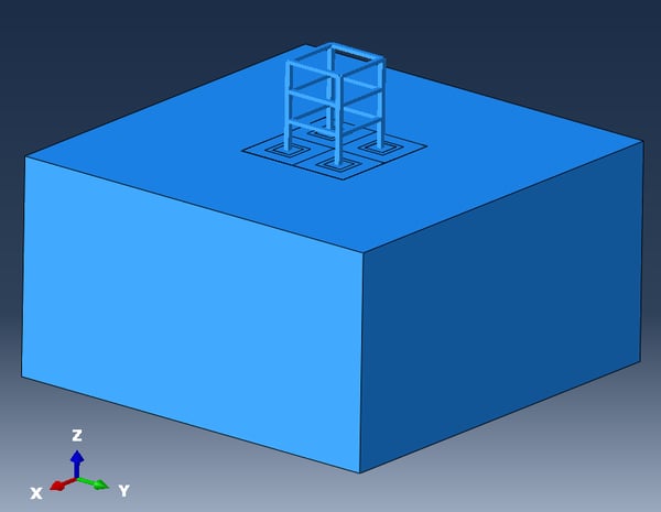
Figure 6: Assembly.
When every part is meshed and all the parts are properly assembled, the merge instances command is performed in order to accommodate the creation of a uniform compatible mesh for the entirety of the assembly. Alternatively proper tie constraints should be imposed on the mesh boundaries. A-detail of the final assembly after the merge command has been performed is shown in Figure 7.
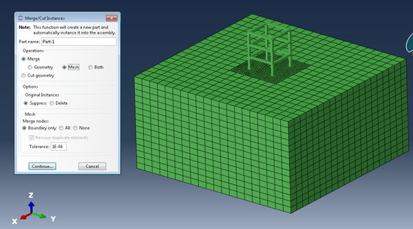
Figure 7: Meshed Assembly and merge instances command.
Soil Block Interactions
In order to guarantee proper soil motion several Multi Point Constraints have been created, to tie the degrees of freedom between the nodes that lie on the same plane (of the soil block). A relevant detail is given in Figure 8.
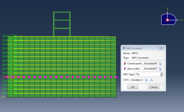
Figure 8: Multi Point constraint detail.
Loads and Boundary Conditions
The lateral (X-axis accelerations) accelerations are applied directly on the lowermost nodes of the soil block. This is done via an imposed acceleration on the X –axis in combination with an amplitude curve definition(“quake”) in order to imposed the recorded acceleration. For the lowermost nodes of the soil block, all displacements are constrained except the X-displacement degree of freedom.
The imposed boundary conditions are shown in Figure 9.
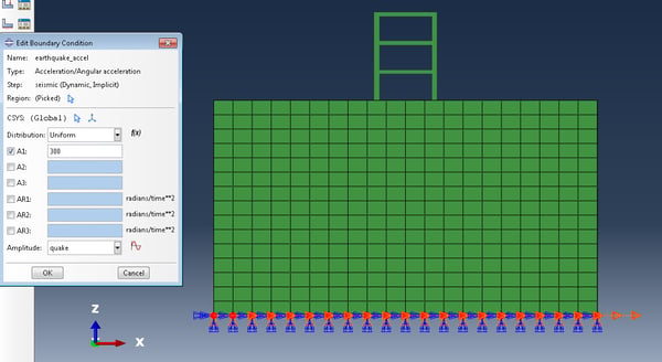
Figure 9: Imposed boundary conditions.
The amplitude curve that was used for this analysis, representing an acceleration history measurement is shown in Figure 10.
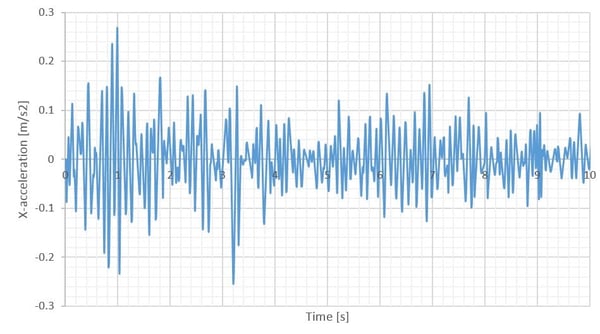
Figure 10: Imposed forcing function of acceleration.
Analysis Settings
For this analysis, a implicit dynamic step has been performed. The step time is equal to 10 seconds with a fixed time increment of 0.01 s to match the acceleration history's frequency.
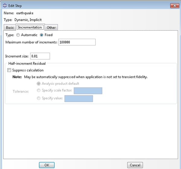
Figure 11: Analysis settings.
Results
What is useful in these types of analyses, is to examine output (e.g. displacement, velocity, acceleration) on a certain point or location of the structure relative to the same output on the base of the structure. This is then called relative output (e.g relative acceleration).
A simple way to do that is to create two different sets , one containing a point located at the highest level of the concrete frame and another set containing a point at the structure’s base, as shown in Figure 12.
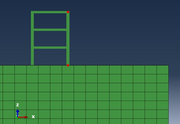
Figure 12: Chosen points for customized history output.
Then the user can request the result values that are of interest by creating history output for both sets.
Then when the respectful output for both sets is available , the user can create a relative output plot, merely by subtracting the output values of the two sets (via XY data--> Operate on XY data--> Dataset point 1 - Dataset point 2).
The lateral displacements (X-axis) of both points of Figure 12 as well as the relative lateral displacements of the uppermoist point of the concrete frame are given in Figure 13.
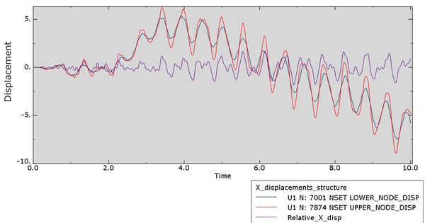
Figure 13: X-displacements and relative X-displacements.
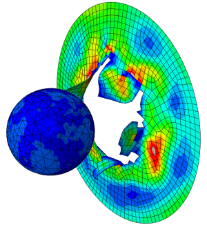
A relevant results video is given below.
Additional Information
Additional modeling details can be incorporated based on the level of detail that the user would like to achieve.
Material damage can be incorporated (e.g. Concrete Damage plasticity) for the concrete frame structure in order to investigate crack initiation.
Soil damage properties with pressure dependence can also be incorporated (e.g. Drucker Prager, Mohr Coulomb).
Material damping in the form of Rayleigh damping (with a and b coefficients) can also be included. A frequency analysis can precede, and based on that certain a and b coefficients can be calculated via known equations (including the values of the extracted eigenfrequencies) and then input in Abaqus in the material property assignments (Materials-->Mechanical--> Damping)


TECHNIA Simulation provides top tier FEA, Non-linear, and Advanced Simulation Software, Training, and Consultancy. Our dedicated team of more than 65 Simulation experts across 16 countries advise and support your innovation with a wealth of specialist knowledge and experience.
About TECHNIA- Related news and articles straight to your inbox
- Hints, tips & how-tos
- Thought leadership articles

Helping you find the information you’re looking for. Discover webinars, events, FAQ's, case studies and tutorials.
VIEW HUB