Modelling Crack Propagation Using XFEM

In a previous blog I showed how to model a stationary crack and calculate the J-integral to determine whether the crack propagates. Abaqus offers different techniques to simulate crack propagation, including surface- and element-based cohesive behaviour and the virtual crack closure technique. When using one of these methods with conventional FEM, the location of the crack needs to be prescribed beforehand. When the eXtended Finite Element Method (XFEM) is used, this is not necessary. In this case, enrichment terms are added to the normal displacement interpolation, so a crack within an element can be described. In this blog I will explain how to model crack propagation using the surface-based cohesive behaviour approach and XFEM.

As an example, loading will be applied to a gear, similar to the stationary crack example. Only in this case, no crack will be present initially and it will develop based on the loading.

Meshing

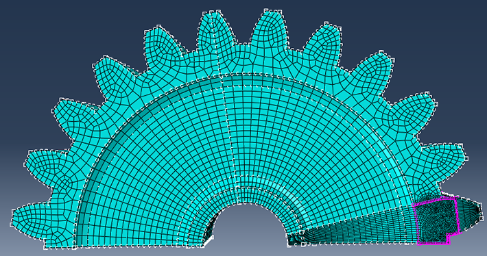
Meshing is much simpler, because it is not necessary to partition an initial crack or circular regions around the crack tip. Partitioning is only used to allow a finer mesh in the region where the crack will develop compared to the rest of the gear. Linear brick elements are used (quadratic elements are not available for XFEM). Half of the gear is modelled, for reasons of symmetry.

Defining Damage – Damage Initiation

To model crack propagation in Abaqus both damage initiation and damage evolution need to be taken into account. Different criteria are available for damage initiation, in this case the maximum principal stress criterion will be used. Compared to criteria based on nominal stress or strain, using the principal stress or strain has the advantage that the crack plane can be perpendicular to the direction of the maximum principal stress, making it solution dependent. Damage initiation is defined as part of the material properties, using damage for Traction Separation laws => Maxps Damage. With this option, damage will initiate when the maximal principal stress exceeds the value given. 

Defining Damage – Damage Evolution

By specifying damage initiation, you do not yet define how the material changes due to damage. Within Abaqus, damage is modelled using a scalar damage parameter, D. This can range between 0 (no damage) and 1 (complete failure). The stress that would have been there without damage is multiplied by (1-D) to calculate the stress including damage. Without damage (D=0) this leads to the undamaged response, with complete failure (D=1) the stress is 0 and in between a fraction of the stress will remain.

In this example, damage is defined using a traction-separation law and damage evolution is a suboption of Maxps Damage.

Either the maximal displacement or the fracture energy, which is the area under the curve in a graph of traction versus separation, must be specified. Different options are possible to specify the softening behaviour: how the traction-separation graph goes from the point at the onset of damage to the completely failed state. In this case linear softening is used, corresponding to a straight line in the traction-separation graph.  It is possible to take into account mode mixing, with the BK law, power law or tabularly specified data. Alternatively, mode-independent behaviour can be specified.

Defining Damage - Damage Stabilization

Simulations including damage evolution often lead to convergence difficulties because of the softening in the material model. Abaqus allows the use of viscous regularization to stabilize the response during damage. For sufficiently small time steps, the tangent stiffness matrix will then be positive definite. A viscosity coefficient can be specified as a suboption of Maxps damage. It should be chosen in such a way that the influence of the stabilization on the final results is small. To check this, the output ALLVD (viscous dissipation) can be compared to ALLSE (strain energy). If ALLVD is not small compared to ALLSE, the viscous stabilization is likely influencing results. Playing around with the viscosity coefficient can help obtain a reasonable result within a reasonable amount of time.

Define Crack

 Apart from defining when the material will damage and how it will behave after damage is initiated, the region where a crack can occur must be specified. This is the region where the enrichment terms will be added. Choosing Special => Crack => Create in the interaction module and selecting the type XFEM in the Create Crack dialog box that appears, allows you to select a crack domain. In this case, the cell where the crack will develop is chosen.

The ‘allow crack growth’ box should be checked, to allow the crack to propagate. XFEM can also be used for stationary cracks, allowing contour integrals such as the J-integral to be calculated with less meshing effort. This is not discussed here. In this example, no initial crack is defined: it will develop based on the damage initiation criterion. If an initial crack is wanted, it is very easy to define with XFEM. A separate part representing the crack (without properties or mesh) can be instanced into the assembly and moved to the correct position. By choosing this part as crack location, the crack is defined. The crack does not need to be along the element edges. In fact, the XFEM method works best if the crack crosses through the element. Frictionless small-sliding contact can be defined for the contact between both sides of the crack.

Solution Controls

To aid in obtaining a converged solution, the solution controls can be modified. From the step module, select other => general solution controls => edit => step in which solution controls are to be edited. Press continue when a warning message is displayed. In the time incrementation tab, discontinuous analysis can be checked. This allows Abaqus to do more iterations before checking whether the solution is going anywhere. In the first More tab, the parameter I­_A can be increased from the default 5, to allow Abaqus more attempts before aborting the simulation. If large cut-backs are required, increasing the number of attempts is useful.

Request Output

For a simulation using XFEM, it is important to request PHILSM as output. This is the signed distance function to describe the crack surface using the level set method. If PHILSM is requested, Abaqus automatically creates an isosurface view cut based on this output, which shows the location of the crack. If it is not requested, the crack will not be visible and results shown will be counterintuitive. STATUSXFEM is also specific for XFEM. It gives the status of the enriched elements, it is 0.0 if the element is undamaged, 1.0 if the element is completely cut through (no traction forces remaining) and a value in between if the element is damaged but some traction forces remain. Of course the normal outputs such as stress and strain are available as well.

Results

With the isosurface view cut based on PHILSM on (default) the results of this simulation nicely show the crack developing in time. By applying translucency, the internal part of the crack is also visible.

 Are you interested to investigate if cracks will cause a potential failure?