
Posted by Simuleon
Table of contents
Previously we posted a blog about optimization of a clap skate using Tosca. I wanted to revisit the topic, by comparing the parametric optimization in Isight and non-parametric optimization in Tosca.
In that blog clap skates were used, but since the weather has started to warm up, I thought in-line skates would be a better case study, particularly the frame (Figure 1). Both software are powerful and complex, so I will try to keep things simple and showcase the basics. More detailed information for the optimization in Isight can be found here and in Tosca here. 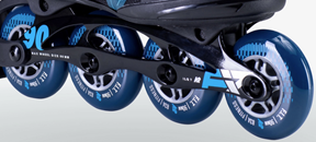
Figure 1. Close-up of an in-line skate frame.
Non-Parametric Optimization
In Tosca, the Topology optimization can be used to generate a proposal for new concept design, based on some predefined criteria. For instance, as an objective we would like to maximize the structural stiffness of the frame. Typically, some constraints are applied, such as the final volume should not be below a certain percentage of the initial volume.
Then the software automatically determines the natural shape to carry the loads while keeping the costs at minimum by removing material where it is not needed. One big advantage of this approach is that there is no need for an existing design and one could start from scratch.
Parametric Optimization
In Isight, the Optimization component tries to find the best design relative to the starting point. For this several key parameters (called design variables) need to be selected and an allowable range for each needs to be defined. Similar to Tosca, an objective function and design constraints are defined. Then, each parameter is varied within the allowable range to find the optimal design. Similarly, we would like to maximize the structural stiffness while minimizing the final volume.
1. Initial Model
Doing some rough measurements of the frame above, we get the following dimensions. The frame is u-shaped with a maximum length of 300mm. The width of the frame is 30mm and the height of 60mm. The mounting holes to the skate boot are 185mm apart. The mounting holes for the wheels are ~95mm apart to accommodate the 90mm wheels. The diameter of the mounting hole is ~2.5mm. An overview of the main dimensions can be seen below in the initial design for Tosca and Isight figures (Figure 2 and Figure 4)
For Tosca, the initial starting point for the frame design are two 300mm x 60mm rectangles, 30mm apart. These are then joined at the top part, where the frame would be mounted to the boot. The mounting holes for the wheels are also included, as these would need to be in the final design. 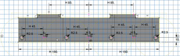
Figure 2. Initial design for the skate frame for Tosca.
A 7075 aluminum alloy material and a constant shell thickness of 5mm were used. The wheels were included as analytical rigids. The frame was then kinematically coupled to each wheel. The top part of the frame was kinematically coupled with a reference point (RP-5), which would correspond to the center of the boot (Figure 3). Then an axial load of 800N was applied, corresponding to an 80kg person fully standing on one leg (i.e. maximum axial load the skate would encounter). Lastly, the reference points of the wheels were kept fixed for all translations.
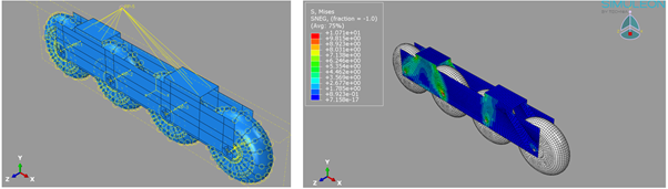
Figure 3. (Left) Assembly and interactions defined for the Tosca optimization. (Right) Results for the initial run.
For Isight, a more complex design was needed including some of the cut-extrusion holes in the frame. For each cut-extrusion, dimensions were defined (Figure 4). Note that the sketch is fully contained, so changing the dimensions in the optimization task in Isight should not produce unrealistic models.
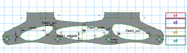
Figure 4. Initial design for the skate frame for Isight.
In this case, the same 7075 aluminum alloy was used. Separate sections were defined for the 4 different regions (Figure 4 – S1 – S4) with a thickness of 3mm for each. The rest of the model is identical to the one from Tosca.
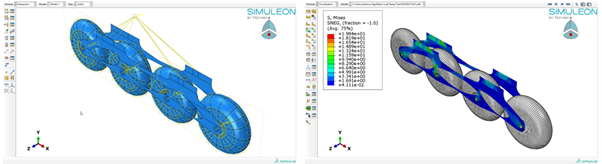
Figure 5. (Left) Assembly and interactions defined for the Isight optimization. (Right) Results for the initial run.
2. Setting Up the Optimization Task in Tosca
The setup of optimization in Tosca was similar previous blogs (i.e. here) with a condition based optimization, minimizing the strain energy as objective (equivalent to maximizing stiffness) and the volume to be contained to 40%. A default 15 cycles was used.
In addition, some regions were frozen, to prevent material removal from regions where they should be present. They were the mounting region to the boot (top part), the mounting holes for the wheels, and the front part of the skate, since the loading used did not produce any stresses in that region. Tosca would just remove this part, since there are not enough loads/boundary conditions to restrict it.
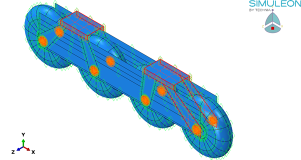
Figure 6. Geometric restrictions (Frozen areas) for Tosca.
3. Setting up the Optimization Task in Isight
In the Process components tab, the default task process was replaced with an optimization process. Then from the Application components tab, Abaqus was included. For Isight, we will further need the .CAE and .ODB files corresponding to the geometry in Figure 4 and Figure 5.
3a. Setting up the Abaqus Component
To set up the Abaqus runs, first we need to define which model Isight will use (Input tab). After reading the .cae file we can select the thicknesses of the shells and the cut-extrusion parameters defined in Figure 4. These will be the variables for the optimization task.
Going to the Execution tab, lets us control which version of Abaqus Isight will use (in this case 2020) and which Output Parameters should be saved (ODB Extraction Options, defaults are used).
Finally, from the Output tab, we select some parameters of interest from the ODB. This is done by first reading the ODB corresponding to the model we are using. In this case, we are interested in the mass, which would then be related to the volume, and the strain energy history output (ALLSE).
3b. Setting up the Optimization Component
In the optimization component setup, in the General tab, we are faced with a wide array of optimization techniques. Luckily, Isight does provide a brief description of each technique and which problems they are best suited for. As this is more of an example, the default NLPQLP technique with 40 iterations was used. As a general note, automatic scaling is enabled. Otherwise, we would have to specify each scaling factor for the parameters.
Now to define the variables, constraints and objectives. For the variables, we activate the parameters obtained from the Abaqus Input component and provide some upper and lower bounds for each variable (Figure 7).
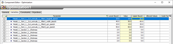
Figure 7. Variable definition
Then, we apply a 40% of mass constraint and we can select the objectives of the optimization. Like Tosca, we would like to minimize the strain energy, thus maximizing the stiffness of the component, while also minimizing the mass.
4. Tosca Results
After 15 cycles, the task is complete. First, we must first combine the optimization results (details here) and the final design cycle is shown below.

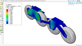
Figure 8. Animation of Tosca results (left). Stresses on the last optimization cycle.
This geometry can now be extracted and used later. For instance, after a topology optimization (assuming the design is final), a sizing optimization could be run to optimize the shell thicknesses.
5. Isight Results
For Isight, we have a few more simulations. Varying each parameter yielded about 233 simulations in total. For each combination of variables tested, we rating the design feasibility and values for the constraint and objective functions. Isight offers many tools to visualize the optimization results.
Since there are quite many, I will just present some main plots:
1) The EDM plot shows on the top the inputs and on the bottom the outputs. For each combination of input parameters (i.e. line on top), we can see the output response (i.e. the line on the bottom).
2) The History plot on the top right size shows the parameter values the optimization process has gone through during the optimization step.
3) The Self-Organizing map on the bottom right size shows the design feasibility. It is a visual way to identify interesting clusters of data and relationships in parameters. For instance, there are several designs with a feasibility of 9.
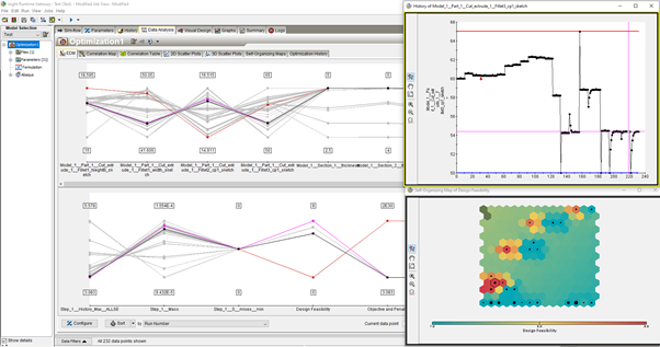
Figure 9. Example graphs for the visualizing the output of the optimization task. (Left) EDM plot; (Top-Right) History output for one of the cut-extrusion variables; (Bottom-Right) Self-organizing map for the design feasibility.
Overall, the result of the Isight optimization provided the following values:
Variable Lower limit Initial Upper limit Optimal (rounded)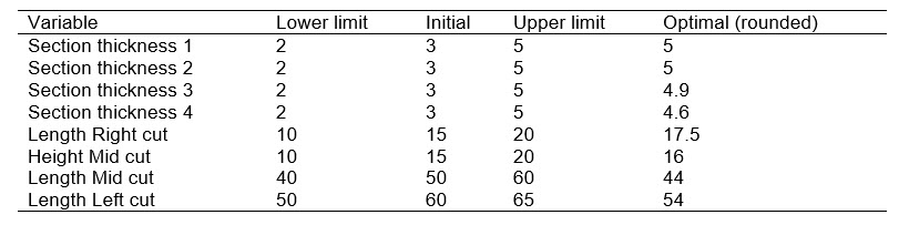
The difference between the initial and final design is visually shown below as well.
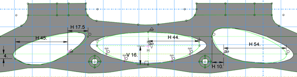
Figure 10. Difference between initial design and final design in terms of extrusion cuts on the frame.
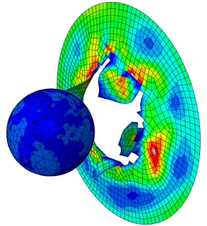
The initial design yielded much higher stresses at the back of the frame, near the boot attachment region, which were minimized in the final design.
Figure 11. Comparison between the initial and optimized results. Note: The vonMises Stress range is identical in both graphs (0-8 MPa).
6. Conclusion
Both types of optimization produce different results and are best suited for different types of applications. Tosca, or non-parametric optimization, is most suited for when there is no initial design and the software can “freely” obtain the optimal configuration. Isight, or parametric optimization, is more suited for optimizing an existing design.
For optimization tasks, it is imperative to have loading and boundary conditions as close to reality as possible. In this case only an axial load was used. More realistically, the forces and motions would be similar to the ones reported for speed skating by researchers at TU Delft and would influence the optimization results and produce a more realistic skate design.


TECHNIA Simulation provides top tier FEA, Non-linear, and Advanced Simulation Software, Training, and Consultancy. Our dedicated team of more than 65 Simulation experts across 16 countries advise and support your innovation with a wealth of specialist knowledge and experience.
About TECHNIA- Related news and articles straight to your inbox
- Hints, tips & how-tos
- Thought leadership articles

Helping you find the information you’re looking for. Discover webinars, events, FAQ's, case studies and tutorials.
VIEW HUB