In the current post, we will be focusing on introducing XFlow CFD by demonstrating an aerodynamic effect primarily observable in spheres or cylinders following certain trajectories while spinning at the same time.

This effect is known as the Magnus effect, associated with spinning objects. A sphere for example travelling through mid-air while spinning at the same time , will drag air faster around one of its sides. This will consequently create a pressure gradient between the sides of the sphere, thus creating a lift force that will alter the sphere’s trajectory compared to a case with no spin.  The lift force generated is equivalent to that of an airfoil, only the origin of the necessary air recirculation around the body is by mechanical rotation (the spin)  and not by aerodynamic design ( the airfoil).

XFlow is a next generation CFD software based on the Lattice-boltzmann method designed for a broad range of computational fluid dynamics simulations. XFlow’s  latest release supports coupling with Abaqus for performing fluid structure interaction analyses.

The Magnus effect will be demonstrated with a spinning football analysis in XFlow.

Preprocessing in XFlow

Herein the setting up of the spinning football analysis will be explained.

In XFlow we will perform  a 3d external type of analysis using a single phase flow model.  The environment ( a segment of a football field in this example) as well as several analysis settings are given in Figure 1.

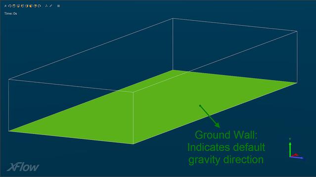
Figure 1: Environment.

Figure 2: Settings.

The analysis type is external because in this way we do not need geometry to define our fluid domain (the football field segment), we can assign its dimensions and position in 3d space directly through the menu, as shown in Figure 2.So our domain type will either be a virtual wind tunnel or a generic rectangular domain ( for the physics and boundary conditions of this analysis, both options are equivalent).

A single phase flow model will be used as a single fluid only (air in this case) will be present inside the fluid domain. Since our analysis is of external type, air properties are automatically assigned to the respectful tab (“ Materials” tab in XFlow). For this analysis gravity was not modelled however acceleration of gravity can be input in the external acceleration laws menu.  The designated turbulence model is set to Automatic. XFlow then assigns the WALE model in order to model turbulence at the football’s boundaries. Turbulence generation is set to off, meaning that no additional turbulence will be introduced at the fluid domain boundaries as an initial condition.

Figure 1 shows the fluid domain, the football field segment, having dimensions of 20x3(height)x8 meters.

In terms of supported geometry for import, all major neutral formats are supported by XFlow (iges, step, stl). Additionally geometry can be designed in Xflow natively.

XFlow also offers the possibility to include geometry for visualization ( post-processing) purposes only. This allows the user to exclude geometries that are of no interest for the cfd analysis –and therefore limit computational effort- while including them  in order to have a  more aesthetically  refined end result.

This is the case for the goal post geometry as indicated in Figure 3.

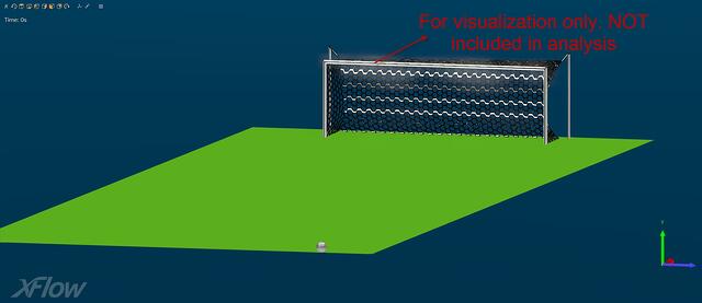
Figure 3: Geometry.

Figure 4. Geometry Settings.

The main geometry of interest in this case will be the football. As was the case with the fluid domain assignment, the geometry can be positioned and oriented at will, inside the fluid domain. For demonstrating the Magnus effect, the ball’s behavor will be set to rigid body dynamics. So the ball will be modelled as fully rigid (non-deformable) and will have all 6 degrees of freedom set to free (set in the  “ constraints” menu), allowing the ball to rotate and displace freely in 3d space. By setting the behavior to rigid body dynamics, the ball’s motion will be influenced by external forces or moments ( the Magnus force produced during ball-air interaction).The user can also assign the mass of the ball directly (as shown in Figure 4).

For the initial conditions of the football’s trajectory, a linear velocity vector is given  as well as an angular Y-axis  velocity, the spin of the football (Figure 4).

Figure 5 shows the domain discretization settings.

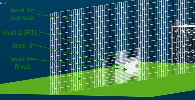
Figure 5: Discretization scheme.

Figure 6: Discretization Settings.

It can be seen that 4 different discretization levels have been assigned. The far field discretization level is the coarsest (level 1). The football is discretized using one fourth of the far field’s discretization and the wake is discretized using one eight of the far field’s discetization. The option for extra refinement at the wake is enabled when the adaptive refinement algorithm is used(as in this analysis). This really efficient algorithm automatically tracks the wake evolution and refines it accordingly, in order to capture it effectively for post processing. An additional refinement level is added(level 2) in order to smoothly transition results between levels 1 and 3(“ refinement transition length” option).

Last but not least, simulation time is set to 2 seconds, based on the football’s velocity and fluid domain dimensions (so that at least the football will cover the full length of the domain) and the time step is manually assigned to  0.005 seconds. This can be modified in order to find the optimum compromise between speeding up the computational time and maintaining the stability factor around 0.3, meaning that the quality of the results is satisfactory.

Post Processing-results

Figure 7 shows the stability parameter for this particular simulation. The values of the stability parameter are within acceptable limits.

Figure 7: Stability Parameter.

A video including the results is included below.

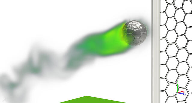
These videos show the vorticity (how much the airflow swirls) of the airflow at the wake of the spinning football , the trajectory curve of the football where the effect of the Magnus force is evident as well as a spin detail of the football, on its way to the spot where even good goalkeepers cannot manage to save it.

As a concluding remark, based on what was demonstrated, it can be seen that XFlow provides superior user friendliness and quickness in setting up even advanced cfd studies. Additionally the lattice discretization scheme overcomes mesh related difficulties of traditional CFD software. Even complex geometries can be included and discretized with a push of a button , reducing mesh generation ( a tedious process inherently present in traditional CFD software) time to a minimum.